Prep regridding input: open RiOMar/GAMAR via Kerchunk → write a temporary Zarr

This notebook prepares a small, reproducible Zarr subset that is fast to iterate on for regridding experiments.

It opens the dataset from a Kerchunk catalog generated on HPC, and the same workflow can open:

directly on the HPC filesystem, or
over HTTPS via the DATARMOR export service (https://data-fair2adapt.ifremer.fr/).

Goal¶

Produce a temporary Zarr (e.g. small.zarr) that is then used as input to:

regrid_apply_ufunc.ipynb

Outputs¶

OUT_ZARR: a lightweight subset written to Zarr (local or HPC scratch)

Steps¶

Open the dataset from a Kerchunk catalog (portable: HPC filesystem or HTTPS export)
Select variables and ensure lon/lat are explicit coordinates
Build a polygon mask helper for the model grid
Define the ROI and apply the mask (load ROI polygon, mask, and subset)
Write a temporary Zarr (e.g. small.zarr) for use by regrid_apply_ufunc.ipynb

Tip: keep this subset small (few timesteps / ROI mask) until the workflow is validated.

Kerchunk catalog options¶

A Kerchunk catalog is a JSON mapping that lets Xarray open a collection of NetCDF (or similar) files as a virtual Zarr dataset.
Depending on where you run this notebook, you can point to:

HPC filesystem path (fast, when you have direct access to /scale/...)
HTTPS export (portable, when you access the same data through https://data-fair2adapt.ifremer.fr/)

Below are example catalog paths that have been created previously (kept here as a reference).

1. Open the dataset from a Kerchunk catalog (portable: HPC filesystem or HTTPS export)¶

Many Kerchunk catalogs store references to the original files (often as absolute HPC paths).
When opening through HTTPS, we rewrite those references from:

/scale/project/lops-oh-fair2adapt/... → https://data-fair2adapt.ifremer.fr/...

The cell below:

Detects whether the HPC path exists (so we are running on the cluster).
Otherwise loads the JSON over HTTPS, patches references in-memory, and opens the dataset.
(Optional) can cache the patched references locally as a parquet file for faster re-opening.

%%time
import json
from pathlib import Path

import fsspec
import xarray as xr

from healpix_regrid import patch_kc_refs_inplace

HPC_PREFIX = "/scale/project/lops-oh-fair2adapt/"
HTTPS_PREFIX = "https://data-fair2adapt.ifremer.fr/"
CATALOG_PATH = "fpaul/tmp/riomar_3months.json"
OUT_PARQUET = "riomar_3months_.parq"  # local parquet refs cache

# ------------------------------
# 1) HPC mode: open directly
# ------------------------------
if Path(HPC_PREFIX).exists():
    KERCHUNK_CATALOG = HPC_PREFIX + CATALOG_PATH
    print("Running in HPC mode:", KERCHUNK_CATALOG)

    ds = xr.open_dataset(KERCHUNK_CATALOG, engine="kerchunk", chunks={})

# ------------------------------
# 2) HTTPS mode: fetch JSON, patch refs, open
# ------------------------------
else:
    KERCHUNK_CATALOG = HTTPS_PREFIX + CATALOG_PATH
    print("Running in HTTPS mode:", KERCHUNK_CATALOG)

    with fsspec.open(KERCHUNK_CATALOG, "rt") as f:
        kc = json.load(f)

    kc = patch_kc_refs_inplace(kc)
    ds = xr.open_dataset(kc, engine="kerchunk", chunks={})

ds

2. Select variables and ensure lon/lat are explicit coordinates¶

The original dataset contains many variables. For this demo we keep:

temp (temperature)
salt (salinity)
zeta (sea surface height)

We also load the 2D longitude/latitude fields and attach them as coordinates (nav_lon_rho, nav_lat_rho).
Loading them explicitly avoids repeated remote reads later (plots, masking, regridding, etc.).

ds = ds[["temp", "salt", "zeta"]].assign_coords(
    nav_lon_rho=ds["nav_lon_rho"].load(),
    nav_lat_rho=ds["nav_lat_rho"].load(),
)
ds

3. Build a polygon mask helper for the model grid¶

To extract a spatial subset, we load a boundary polygon (GeoJSON) and create a boolean mask on the dataset grid:

True → grid point is inside the polygon
False → outside

This is useful to reduce the dataset to a Region Of Interest (ROI) before saving or regridding.

import numpy as np

from healpix_regrid import apply_polygon_mask

4. Define the ROI and apply the mask (load ROI polygon, mask, and subset)¶

For the regridding demo we focus on a limited area defined by an outer boundary polygon (stored in outer_boundary.geojson).
We will:

Read the polygon from GeoJSON.
Trim the dataset in time (keep only a couple of timesteps for a lightweight example).
Add the polygon mask to the dataset.

In the next notebook (e.g. simple_regrid.ipynb) we will use the saved subset for regridding experiments.

import geopandas as gpd

# 1. Read the polygon from GeoJSON.

gdf = gpd.read_file("outer_boundary.geojson", driver="GeoJSON")
poly = gdf.geometry.iloc[0]

# 2. Trim the dataset in time
# (keep only a couple of timesteps for a lightweight example).
ds = ds.isel(time_counter=slice(0, 2))[["temp", "salt", "zeta"]]

# 3. Add the polygon mask to the dataset.

ds_temp = apply_polygon_mask(ds, poly)
ds_temp

Inspect the native grid extent for plotting

After applying the ROI mask, we compute the min/max longitude/latitude of valid grid points.
This helps confirm we are working on the expected geographic area and can be used to set plot limits.

lat = ds_temp["nav_lat_rho"]
lon = ds_temp["nav_lon_rho"]

valid = (lat != -1) & (lon != -1)  # or (lat > -90) & (lon > -180) if you prefer

lat_min = lat.where(valid).min().item()
lat_max = lat.where(valid).max().item()
lon_min = lon.where(valid).min().item()
lon_max = lon.where(valid).max().item()

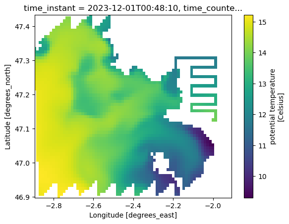
lat_min, lat_max, lon_min, lon_max

(46.89809036254883, 47.4329719543457, -2.8933334350585938, -1.90666663646698)

Quick visual check

Plot one surface slice (time_counter=0, s_rho=0) to verify that:

coordinates are correctly attached (nav_lon_rho, nav_lat_rho)
the selected subset matches the intended area

ds_temp.temp.isel(time_counter=0, s_rho=0).plot(
    y="nav_lat_rho", x="nav_lon_rho", ylim=(lat_min, lat_max), xlim=(lon_min, lon_max)
)

5. Write a temporary Zarr (e.g. `small.zarr`) for use by `regrid_apply_ufunc.ipynb`¶

To make the next steps (regridding) fast and reproducible, we write the masked / subsetted dataset to a local Zarr store.

Tip: adjust OUT_ZARR to a location that exists on your machine (or to a shared scratch directory on HPC).

%%time
OUT_ZARR = "/Users/todaka/data/RIOMAR/small.zarr"
ds_temp.to_zarr(OUT_ZARR, mode="w")

/Users/todaka/micromamba/envs/pangeo/lib/python3.13/site-packages/zarr/api/asynchronous.py:247: ZarrUserWarning: Consolidated metadata is currently not part in the Zarr format 3 specification. It may not be supported by other zarr implementations and may change in the future.
  warnings.warn(

CPU times: user 12.7 s, sys: 7.4 s, total: 20.1 s
Wall time: 1min 56s

<xarray.backends.zarr.ZarrStore at 0x13ff727a0>

Re-open the Zarr subset and plot

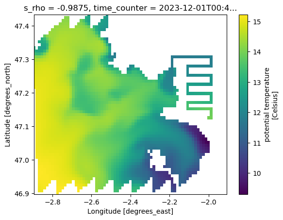
This verifies that the data were written correctly and can be opened independently of the original Kerchunk catalog.

%%time
OUT_ZARR = "/Users/todaka/data/RIOMAR/small.zarr"

small_ds = xr.open_zarr(OUT_ZARR)

small_ds.temp.isel(time_counter=0, s_rho=0).plot(
    y="nav_lat_rho", x="nav_lon_rho", ylim=(lat_min, lat_max), xlim=(lon_min, lon_max)
)

CPU times: user 40.3 ms, sys: 8.61 ms, total: 48.9 ms
Wall time: 48.4 ms

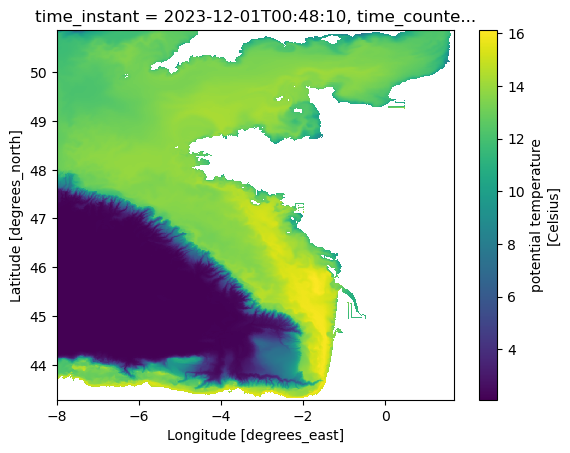
Optional: broader view

A second plot with wider latitude limits can help spot any unexpected artifacts (e.g., missing values, wrap-around).

lat = ds["nav_lat_rho"]
lon = ds["nav_lon_rho"]

valid = (lat != -1) & (lon != -1)  # or (lat > -90) & (lon > -180) if you prefer

lat_min = lat.where(valid).min().item()
lat_max = lat.where(valid).max().item()
lon_min = lon.where(valid).min().item()
lon_max = lon.where(valid).max().item()

ds.temp.isel(time_counter=0, s_rho=0).plot(
    y="nav_lat_rho", x="nav_lon_rho", ylim=(lat_min, lat_max), xlim=(lon_min, lon_max)
)

(Optional) Convert ROI data to an XDGGs / HEALPix-indexed DataArray

If your next step is to move from the native model grid to a DGGS representation (e.g. HEALPix), it can be convenient to store values against a cell_ids index.

The helper below builds an xarray.DataArray that follows the metadata conventions expected by xdggs. You can then attach this to a dataset, write it to Zarr, or use it in downstream regridding/resampling code.

import xarray as xr
import xdggs


def make_xdggs_dataarray_from_cell_ids(
    data,
    cell_ids,
    level: int = 15,
    name: str = "da",
):
    """
    Build an xdggs-compatible DataArray indexed by HEALPix `cell_ids`.

    Parameters
    ----------
    data : array-like
        Values for each cell (same length as `cell_ids`).
    cell_ids : array-like of int
        HEALPix cell identifiers (nested indexing).
    level : int
        HEALPix resolution level.
    name : str
        Name of the DataArray.

    Returns
    -------
    xr.DataArray
        Decoded and enriched with latitude/longitude coordinates via xdggs.
    """
    cell_ids = np.asarray(cell_ids, dtype=np.int64)

    da = xr.DataArray(
        data,
        dims=("cell_ids",),
        coords={"cell_ids": ("cell_ids", cell_ids)},
        name=name,
    )

    # Minimal metadata expected by xdggs
    da["cell_ids"].attrs.update(
        {
            "grid_name": "healpix",
            "level": int(level),
            "indexing_scheme": "nested",
            "ellipsoid": "WGS84",
        }
    )

    # Decode -> attach DGGS accessor -> compute lat/lon coordinates
    return da.pipe(xdggs.decode).dggs.assign_latlon_coords()


with np.load("parent_ids.npz") as data:
    parent_ids = data["parent_ids"]
    parent_level = int(data["parent_level"])

da_hp = make_xdggs_dataarray_from_cell_ids(
    np.ones(len(parent_ids)), parent_ids, level=parent_level
)
da_hp.dggs.explore(alpha=0.3)