FAIR2Adapt Case study 1 (CS1) sample dataset#
Context#
Purpose#
The FAIR2Adapt CS1 “Spread of radioactive isotopes in the Arctic under different climate scenarios to understand the climate change impact on radionuclide distribution for public and environmental safety” is owned by NERSC (Norway). The goal is to get familiar with this type of data.
Description#
In this notebook, we will:
Open datasets (DOI: 10.11582/2024.00093) that were downloaded from the NIRD archive and deposited in the EOSC bucket of FAIR2Adapt
Check some metadata and select a variable to plot.
Contributions#
Notebook#
Anne Fouilloux, Simula Research Laboratory (Norway) (author), @annefou
Even Moa Myklebust, Simula Research Laboratory (Norway) (reviewer), @evenmm
Bibliography and other interesting resources#
NorESM dataset used in this notebook, 10.11582/2024.00093
Import Libraries#
import s3fs
import xarray as xr
import matplotlib.pyplot as plt
import cartopy.crs as ccrs
Open one history file from the Ocean (MICOM model) component#
client_kwargs={'endpoint_url': 'https://pangeo-eosc-minioapi.vm.fedcloud.eu/'}


s3 = s3fs.S3FileSystem(anon=True, client_kwargs=client_kwargs)

filename = "s3://afouilloux-fair2adapt/10.11582_2024.00093/N1850_f19_tn14_20190722/ocn/hist/N1850_f19_tn14_20190722.micom.hbgcd.1801-01.nc"

s3.ls(filename)
['afouilloux-fair2adapt/10.11582_2024.00093/N1850_f19_tn14_20190722/ocn/hist/N1850_f19_tn14_20190722.micom.hbgcd.1801-01.nc']
ds = xr.open_dataset(s3.open(filename))
ds
<xarray.Dataset> Size: 103MB
Dimensions:     (time: 31, sigma: 53, depth: 70, bounds: 2, y: 385, x: 360)
Coordinates:
  * time        (time) object 248B 1801-01-01 12:00:00 ... 1801-01-31 12:00:00
  * sigma       (sigma) float64 424B 27.22 27.72 28.2 28.68 ... 37.48 37.58 37.8
  * depth       (depth) float64 560B 0.0 5.0 10.0 ... 6.25e+03 6.5e+03 6.75e+03
Dimensions without coordinates: bounds, y, x
Data variables:
    depth_bnds  (depth, bounds) float64 1kB ...
    co2fxd      (time, y, x) float32 17MB ...
    co2fxu      (time, y, x) float32 17MB ...
    srfdissic   (time, y, x) float32 17MB ...
    srftalk     (time, y, x) float32 17MB ...
    srfphyc     (time, y, x) float32 17MB ...
    ppint       (time, y, x) float32 17MB ...
xarray.Dataset
- time: 31
- sigma: 53
- depth: 70
- bounds: 2
- y: 385
- x: 360
- time(time)object1801-01-01 12:00:00 ... 1801-01-...
- long_name :
- time
array([cftime.DatetimeNoLeap(1801, 1, 1, 12, 0, 0, 0, has_year_zero=True), cftime.DatetimeNoLeap(1801, 1, 2, 12, 0, 0, 0, has_year_zero=True), cftime.DatetimeNoLeap(1801, 1, 3, 12, 0, 0, 0, has_year_zero=True), cftime.DatetimeNoLeap(1801, 1, 4, 12, 0, 0, 0, has_year_zero=True), cftime.DatetimeNoLeap(1801, 1, 5, 12, 0, 0, 0, has_year_zero=True), cftime.DatetimeNoLeap(1801, 1, 6, 12, 0, 0, 0, has_year_zero=True), cftime.DatetimeNoLeap(1801, 1, 7, 12, 0, 0, 0, has_year_zero=True), cftime.DatetimeNoLeap(1801, 1, 8, 12, 0, 0, 0, has_year_zero=True), cftime.DatetimeNoLeap(1801, 1, 9, 12, 0, 0, 0, has_year_zero=True), cftime.DatetimeNoLeap(1801, 1, 10, 12, 0, 0, 0, has_year_zero=True), cftime.DatetimeNoLeap(1801, 1, 11, 12, 0, 0, 0, has_year_zero=True), cftime.DatetimeNoLeap(1801, 1, 12, 12, 0, 0, 0, has_year_zero=True), cftime.DatetimeNoLeap(1801, 1, 13, 12, 0, 0, 0, has_year_zero=True), cftime.DatetimeNoLeap(1801, 1, 14, 12, 0, 0, 0, has_year_zero=True), cftime.DatetimeNoLeap(1801, 1, 15, 12, 0, 0, 0, has_year_zero=True), cftime.DatetimeNoLeap(1801, 1, 16, 12, 0, 0, 0, has_year_zero=True), cftime.DatetimeNoLeap(1801, 1, 17, 12, 0, 0, 0, has_year_zero=True), cftime.DatetimeNoLeap(1801, 1, 18, 12, 0, 0, 0, has_year_zero=True), cftime.DatetimeNoLeap(1801, 1, 19, 12, 0, 0, 0, has_year_zero=True), cftime.DatetimeNoLeap(1801, 1, 20, 12, 0, 0, 0, has_year_zero=True), cftime.DatetimeNoLeap(1801, 1, 21, 12, 0, 0, 0, has_year_zero=True), cftime.DatetimeNoLeap(1801, 1, 22, 12, 0, 0, 0, has_year_zero=True), cftime.DatetimeNoLeap(1801, 1, 23, 12, 0, 0, 0, has_year_zero=True), cftime.DatetimeNoLeap(1801, 1, 24, 12, 0, 0, 0, has_year_zero=True), cftime.DatetimeNoLeap(1801, 1, 25, 12, 0, 0, 0, has_year_zero=True), cftime.DatetimeNoLeap(1801, 1, 26, 12, 0, 0, 0, has_year_zero=True), cftime.DatetimeNoLeap(1801, 1, 27, 12, 0, 0, 0, has_year_zero=True), cftime.DatetimeNoLeap(1801, 1, 28, 12, 0, 0, 0, has_year_zero=True), cftime.DatetimeNoLeap(1801, 1, 29, 12, 0, 0, 0, has_year_zero=True), cftime.DatetimeNoLeap(1801, 1, 30, 12, 0, 0, 0, has_year_zero=True), cftime.DatetimeNoLeap(1801, 1, 31, 12, 0, 0, 0, has_year_zero=True)], dtype=object) - sigma(sigma)float6427.22 27.72 28.2 ... 37.58 37.8
- long_name :
- Potential density
- standard_name :
- sea_water_sigma_theta
- units :
- kg m-3
- positive :
- down
array([27.22 , 27.72 , 28.202, 28.681, 29.158, 29.632, 30.102, 30.567, 31.026, 31.477, 31.92 , 32.352, 32.772, 33.176, 33.564, 33.932, 34.279, 34.602, 34.9 , 35.172, 35.417, 35.637, 35.832, 36.003, 36.153, 36.284, 36.398, 36.497, 36.584, 36.66 , 36.728, 36.789, 36.843, 36.893, 36.939, 36.982, 37.022, 37.06 , 37.096, 37.131, 37.166, 37.199, 37.231, 37.264, 37.295, 37.327, 37.358, 37.388, 37.419, 37.45 , 37.48 , 37.58 , 37.8 ]) - depth(depth)float640.0 5.0 10.0 ... 6.5e+03 6.75e+03
- long_name :
- z level
- units :
- m
- positive :
- down
- bounds :
- depth_bnds
array([0.000e+00, 5.000e+00, 1.000e+01, 1.500e+01, 2.000e+01, 2.500e+01,
       3.000e+01, 4.000e+01, 5.000e+01, 6.250e+01, 7.500e+01, 8.750e+01,
       1.000e+02, 1.125e+02, 1.250e+02, 1.375e+02, 1.500e+02, 1.750e+02,
       2.000e+02, 2.250e+02, 2.500e+02, 2.750e+02, 3.000e+02, 3.500e+02,
       4.000e+02, 4.500e+02, 5.000e+02, 5.500e+02, 6.000e+02, 6.500e+02,
       7.000e+02, 7.500e+02, 8.000e+02, 8.500e+02, 9.000e+02, 9.500e+02,
       1.000e+03, 1.050e+03, 1.100e+03, 1.150e+03, 1.200e+03, 1.250e+03,
       1.300e+03, 1.350e+03, 1.400e+03, 1.450e+03, 1.500e+03, 1.625e+03,
       1.750e+03, 1.875e+03, 2.000e+03, 2.250e+03, 2.500e+03, 2.750e+03,
       3.000e+03, 3.250e+03, 3.500e+03, 3.750e+03, 4.000e+03, 4.250e+03,
       4.500e+03, 4.750e+03, 5.000e+03, 5.250e+03, 5.500e+03, 5.750e+03,
       6.000e+03, 6.250e+03, 6.500e+03, 6.750e+03])
- depth_bnds(depth, bounds)float64...
[140 values with dtype=float64]
- co2fxd(time, y, x)float32...
- units :
- kg C m-2 s-1
- long_name :
- Downward CO2 flux
- cell_measures :
- area: parea
[4296600 values with dtype=float32]
- co2fxu(time, y, x)float32...
- units :
- kg C m-2 s-1
- long_name :
- Upward CO2 flux
- cell_measures :
- area: parea
[4296600 values with dtype=float32]
- srfdissic(time, y, x)float32...
- units :
- mol C m-3
- long_name :
- Surface dissolved inorganic carbon
- cell_measures :
- area: parea
[4296600 values with dtype=float32]
- srftalk(time, y, x)float32...
- units :
- eq m-3
- long_name :
- Surface alkalinity
- cell_measures :
- area: parea
[4296600 values with dtype=float32]
- srfphyc(time, y, x)float32...
- units :
- mol P m-3
- long_name :
- Surface phytoplankton
- cell_measures :
- area: parea
[4296600 values with dtype=float32]
- ppint(time, y, x)float32...
- units :
- mol C m-2 s-1
- long_name :
- Integrated primary production
- cell_measures :
- area: parea
[4296600 values with dtype=float32]
- timePandasIndex
PandasIndex(CFTimeIndex([1801-01-01 12:00:00, 1801-01-02 12:00:00, 1801-01-03 12:00:00, 1801-01-04 12:00:00, 1801-01-05 12:00:00, 1801-01-06 12:00:00, 1801-01-07 12:00:00, 1801-01-08 12:00:00, 1801-01-09 12:00:00, 1801-01-10 12:00:00, 1801-01-11 12:00:00, 1801-01-12 12:00:00, 1801-01-13 12:00:00, 1801-01-14 12:00:00, 1801-01-15 12:00:00, 1801-01-16 12:00:00, 1801-01-17 12:00:00, 1801-01-18 12:00:00, 1801-01-19 12:00:00, 1801-01-20 12:00:00, 1801-01-21 12:00:00, 1801-01-22 12:00:00, 1801-01-23 12:00:00, 1801-01-24 12:00:00, 1801-01-25 12:00:00, 1801-01-26 12:00:00, 1801-01-27 12:00:00, 1801-01-28 12:00:00, 1801-01-29 12:00:00, 1801-01-30 12:00:00, 1801-01-31 12:00:00], dtype='object', length=31, calendar='noleap', freq='D')) - sigmaPandasIndex
PandasIndex(Index([ 27.22, 27.72, 28.202, 28.681, 29.158, 29.632, 30.102, 30.567, 31.026, 31.477, 31.92, 32.352, 32.772, 33.176, 33.564, 33.932, 34.279, 34.602, 34.9, 35.172, 35.417, 35.637, 35.832, 36.003, 36.153, 36.284, 36.398, 36.497, 36.584, 36.66, 36.728, 36.789, 36.843, 36.893, 36.939, 36.982, 37.022, 37.06, 37.096, 37.131, 37.166, 37.199, 37.231, 37.264, 37.295, 37.327, 37.358, 37.388, 37.419, 37.45, 37.48, 37.58, 37.8], dtype='float64', name='sigma')) - depthPandasIndex
PandasIndex(Index([   0.0,    5.0,   10.0,   15.0,   20.0,   25.0,   30.0,   40.0,   50.0,
         62.5,   75.0,   87.5,  100.0,  112.5,  125.0,  137.5,  150.0,  175.0,
        200.0,  225.0,  250.0,  275.0,  300.0,  350.0,  400.0,  450.0,  500.0,
        550.0,  600.0,  650.0,  700.0,  750.0,  800.0,  850.0,  900.0,  950.0,
       1000.0, 1050.0, 1100.0, 1150.0, 1200.0, 1250.0, 1300.0, 1350.0, 1400.0,
       1450.0, 1500.0, 1625.0, 1750.0, 1875.0, 2000.0, 2250.0, 2500.0, 2750.0,
       3000.0, 3250.0, 3500.0, 3750.0, 4000.0, 4250.0, 4500.0, 4750.0, 5000.0,
       5250.0, 5500.0, 5750.0, 6000.0, 6250.0, 6500.0, 6750.0],
      dtype='float64', name='depth'))
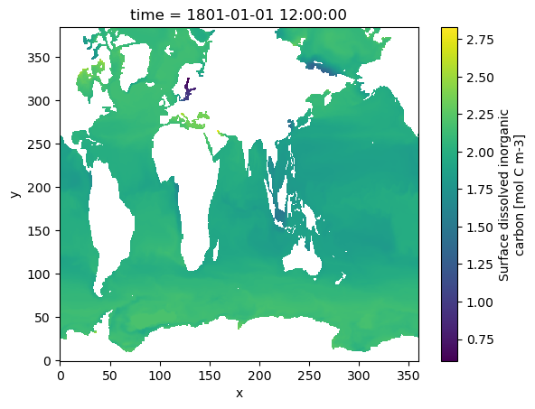
Simple plot of one variable (Surface dissolved inorganic carbon)#
ds.srfdissic
<xarray.DataArray 'srfdissic' (time: 31, y: 385, x: 360)> Size: 17MB
[4296600 values with dtype=float32]
Coordinates:
  * time     (time) object 248B 1801-01-01 12:00:00 ... 1801-01-31 12:00:00
Dimensions without coordinates: y, x
Attributes:
    units:          mol C m-3
    long_name:      Surface dissolved inorganic carbon
    cell_measures:  area: parea
xarray.DataArray
'srfdissic'
- time: 31
- y: 385
- x: 360
- ...
[4296600 values with dtype=float32]
- time(time)object1801-01-01 12:00:00 ... 1801-01-...
- long_name :
- time
array([cftime.DatetimeNoLeap(1801, 1, 1, 12, 0, 0, 0, has_year_zero=True),
       cftime.DatetimeNoLeap(1801, 1, 2, 12, 0, 0, 0, has_year_zero=True),
       cftime.DatetimeNoLeap(1801, 1, 3, 12, 0, 0, 0, has_year_zero=True),
       cftime.DatetimeNoLeap(1801, 1, 4, 12, 0, 0, 0, has_year_zero=True),
       cftime.DatetimeNoLeap(1801, 1, 5, 12, 0, 0, 0, has_year_zero=True),
       cftime.DatetimeNoLeap(1801, 1, 6, 12, 0, 0, 0, has_year_zero=True),
       cftime.DatetimeNoLeap(1801, 1, 7, 12, 0, 0, 0, has_year_zero=True),
       cftime.DatetimeNoLeap(1801, 1, 8, 12, 0, 0, 0, has_year_zero=True),
       cftime.DatetimeNoLeap(1801, 1, 9, 12, 0, 0, 0, has_year_zero=True),
       cftime.DatetimeNoLeap(1801, 1, 10, 12, 0, 0, 0, has_year_zero=True),
       cftime.DatetimeNoLeap(1801, 1, 11, 12, 0, 0, 0, has_year_zero=True),
       cftime.DatetimeNoLeap(1801, 1, 12, 12, 0, 0, 0, has_year_zero=True),
       cftime.DatetimeNoLeap(1801, 1, 13, 12, 0, 0, 0, has_year_zero=True),
       cftime.DatetimeNoLeap(1801, 1, 14, 12, 0, 0, 0, has_year_zero=True),
       cftime.DatetimeNoLeap(1801, 1, 15, 12, 0, 0, 0, has_year_zero=True),
       cftime.DatetimeNoLeap(1801, 1, 16, 12, 0, 0, 0, has_year_zero=True),
       cftime.DatetimeNoLeap(1801, 1, 17, 12, 0, 0, 0, has_year_zero=True),
       cftime.DatetimeNoLeap(1801, 1, 18, 12, 0, 0, 0, has_year_zero=True),
       cftime.DatetimeNoLeap(1801, 1, 19, 12, 0, 0, 0, has_year_zero=True),
       cftime.DatetimeNoLeap(1801, 1, 20, 12, 0, 0, 0, has_year_zero=True),
       cftime.DatetimeNoLeap(1801, 1, 21, 12, 0, 0, 0, has_year_zero=True),
       cftime.DatetimeNoLeap(1801, 1, 22, 12, 0, 0, 0, has_year_zero=True),
       cftime.DatetimeNoLeap(1801, 1, 23, 12, 0, 0, 0, has_year_zero=True),
       cftime.DatetimeNoLeap(1801, 1, 24, 12, 0, 0, 0, has_year_zero=True),
       cftime.DatetimeNoLeap(1801, 1, 25, 12, 0, 0, 0, has_year_zero=True),
       cftime.DatetimeNoLeap(1801, 1, 26, 12, 0, 0, 0, has_year_zero=True),
       cftime.DatetimeNoLeap(1801, 1, 27, 12, 0, 0, 0, has_year_zero=True),
       cftime.DatetimeNoLeap(1801, 1, 28, 12, 0, 0, 0, has_year_zero=True),
       cftime.DatetimeNoLeap(1801, 1, 29, 12, 0, 0, 0, has_year_zero=True),
       cftime.DatetimeNoLeap(1801, 1, 30, 12, 0, 0, 0, has_year_zero=True),
       cftime.DatetimeNoLeap(1801, 1, 31, 12, 0, 0, 0, has_year_zero=True)],
      dtype=object)
- timePandasIndex
PandasIndex(CFTimeIndex([1801-01-01 12:00:00, 1801-01-02 12:00:00, 1801-01-03 12:00:00,
             1801-01-04 12:00:00, 1801-01-05 12:00:00, 1801-01-06 12:00:00,
             1801-01-07 12:00:00, 1801-01-08 12:00:00, 1801-01-09 12:00:00,
             1801-01-10 12:00:00, 1801-01-11 12:00:00, 1801-01-12 12:00:00,
             1801-01-13 12:00:00, 1801-01-14 12:00:00, 1801-01-15 12:00:00,
             1801-01-16 12:00:00, 1801-01-17 12:00:00, 1801-01-18 12:00:00,
             1801-01-19 12:00:00, 1801-01-20 12:00:00, 1801-01-21 12:00:00,
             1801-01-22 12:00:00, 1801-01-23 12:00:00, 1801-01-24 12:00:00,
             1801-01-25 12:00:00, 1801-01-26 12:00:00, 1801-01-27 12:00:00,
             1801-01-28 12:00:00, 1801-01-29 12:00:00, 1801-01-30 12:00:00,
             1801-01-31 12:00:00],
            dtype='object', length=31, calendar='noleap', freq='D'))
- units :
- mol C m-3
- long_name :
- Surface dissolved inorganic carbon
- cell_measures :
- area: parea
ds.srfdissic.isel(time=0).plot()
<matplotlib.collections.QuadMesh at 0x6ffc1083fb90>
Open one history file from the Atmosphere component#
filename = "s3://afouilloux-fair2adapt/10.11582_2024.00093/N1850_f19_tn14_20190722/atm/hist/N1850_f19_tn14_20190722.cam.h0.1801-01.nc"
ds = xr.open_dataset(s3.open(filename))
ds
<xarray.Dataset> Size: 583MB
Dimensions:               (lat: 96, zlon: 1, nbnd: 2, lon: 144, lev: 32,
                           ilev: 33, time: 1)
Coordinates:
  * lat                   (lat) float64 768B -90.0 -88.11 -86.21 ... 88.11 90.0
  * zlon                  (zlon) float64 8B 0.0
  * lon                   (lon) float64 1kB 0.0 2.5 5.0 ... 352.5 355.0 357.5
  * lev                   (lev) float64 256B 3.643 7.595 14.36 ... 976.3 992.6
  * ilev                  (ilev) float64 264B 2.255 5.032 10.16 ... 985.1 1e+03
  * time                  (time) object 8B 1801-02-01 00:00:00
Dimensions without coordinates: nbnd
Data variables: (12/1194)
    zlon_bnds             (zlon, nbnd) float64 16B ...
    gw                    (lat) float64 768B ...
    hyam                  (lev) float64 256B ...
    hybm                  (lev) float64 256B ...
    P0                    float64 8B ...
    hyai                  (ilev) float64 264B ...
    ...                    ...
    mmr_OM                (time, lev, lat, lon) float32 2MB ...
    mmr_SALT              (time, lev, lat, lon) float32 2MB ...
    mmr_SULFATE           (time, lev, lat, lon) float32 2MB ...
    monoterp              (time, lev, lat, lon) float32 2MB ...
    monoterp_SRF          (time, lat, lon) float32 55kB ...
    ozone                 (time, lev, lat, lon) float32 2MB ...
Attributes:
    Conventions:       CF-1.0
    source:            CAM
    case:              N1850_f19_tn14_20190722
    logname:           olivie
    host:
    initial_file:      /cluster/shared/noresm/inputdata/atm/cam/inic/fv/cami-...
    topography_file:   /cluster/shared/noresm/inputdata/atm/cam/topo/fv_1.9x2...
    model_doi_url:     https://doi.org/10.5065/D67H1H0V
    time_period_freq:  month_1
xarray.Dataset
- lat: 96
- zlon: 1
- nbnd: 2
- lon: 144
- lev: 32
- ilev: 33
- time: 1
- lat(lat)float64-90.0 -88.11 -86.21 ... 88.11 90.0
- long_name :
- latitude
- units :
- degrees_north
array([-90. , -88.105263, -86.210526, -84.315789, -82.421053, -80.526316, -78.631579, -76.736842, -74.842105, -72.947368, -71.052632, -69.157895, -67.263158, -65.368421, -63.473684, -61.578947, -59.684211, -57.789474, -55.894737, -54. , -52.105263, -50.210526, -48.315789, -46.421053, -44.526316, -42.631579, -40.736842, -38.842105, -36.947368, -35.052632, -33.157895, -31.263158, -29.368421, -27.473684, -25.578947, -23.684211, -21.789474, -19.894737, -18. , -16.105263, -14.210526, -12.315789, -10.421053, -8.526316, -6.631579, -4.736842, -2.842105, -0.947368, 0.947368, 2.842105, 4.736842, 6.631579, 8.526316, 10.421053, 12.315789, 14.210526, 16.105263, 18. , 19.894737, 21.789474, 23.684211, 25.578947, 27.473684, 29.368421, 31.263158, 33.157895, 35.052632, 36.947368, 38.842105, 40.736842, 42.631579, 44.526316, 46.421053, 48.315789, 50.210526, 52.105263, 54. , 55.894737, 57.789474, 59.684211, 61.578947, 63.473684, 65.368421, 67.263158, 69.157895, 71.052632, 72.947368, 74.842105, 76.736842, 78.631579, 80.526316, 82.421053, 84.315789, 86.210526, 88.105263, 90. ]) - zlon(zlon)float640.0
- long_name :
- longitude
- units :
- degrees_east
- bounds :
- zlon_bnds
array([0.])
- lon(lon)float640.0 2.5 5.0 ... 352.5 355.0 357.5
- long_name :
- longitude
- units :
- degrees_east
array([ 0. , 2.5, 5. , 7.5, 10. , 12.5, 15. , 17.5, 20. , 22.5, 25. , 27.5, 30. , 32.5, 35. , 37.5, 40. , 42.5, 45. , 47.5, 50. , 52.5, 55. , 57.5, 60. , 62.5, 65. , 67.5, 70. , 72.5, 75. , 77.5, 80. , 82.5, 85. , 87.5, 90. , 92.5, 95. , 97.5, 100. , 102.5, 105. , 107.5, 110. , 112.5, 115. , 117.5, 120. , 122.5, 125. , 127.5, 130. , 132.5, 135. , 137.5, 140. , 142.5, 145. , 147.5, 150. , 152.5, 155. , 157.5, 160. , 162.5, 165. , 167.5, 170. , 172.5, 175. , 177.5, 180. , 182.5, 185. , 187.5, 190. , 192.5, 195. , 197.5, 200. , 202.5, 205. , 207.5, 210. , 212.5, 215. , 217.5, 220. , 222.5, 225. , 227.5, 230. , 232.5, 235. , 237.5, 240. , 242.5, 245. , 247.5, 250. , 252.5, 255. , 257.5, 260. , 262.5, 265. , 267.5, 270. , 272.5, 275. , 277.5, 280. , 282.5, 285. , 287.5, 290. , 292.5, 295. , 297.5, 300. , 302.5, 305. , 307.5, 310. , 312.5, 315. , 317.5, 320. , 322.5, 325. , 327.5, 330. , 332.5, 335. , 337.5, 340. , 342.5, 345. , 347.5, 350. , 352.5, 355. , 357.5]) - lev(lev)float643.643 7.595 14.36 ... 976.3 992.6
- long_name :
- hybrid level at midpoints (1000*(A+B))
- units :
- hPa
- positive :
- down
- standard_name :
- atmosphere_hybrid_sigma_pressure_coordinate
- formula_terms :
- a: hyam b: hybm p0: P0 ps: PS
array([ 3.643466, 7.59482 , 14.356632, 24.61222 , 35.92325 , 43.19375 , 51.677499, 61.520498, 73.750958, 87.82123 , 103.317127, 121.547241, 142.994039, 168.22508 , 197.908087, 232.828619, 273.910817, 322.241902, 379.100904, 445.992574, 524.687175, 609.778695, 691.38943 , 763.404481, 820.858369, 859.534767, 887.020249, 912.644547, 936.198398, 957.48548 , 976.325407, 992.556095]) - ilev(ilev)float642.255 5.032 10.16 ... 985.1 1e+03
- long_name :
- hybrid level at interfaces (1000*(A+B))
- units :
- hPa
- positive :
- down
- standard_name :
- atmosphere_hybrid_sigma_pressure_coordinate
- formula_terms :
- a: hyai b: hybi p0: P0 ps: PS
array([ 2.25524 , 5.031692, 10.157947, 18.555317, 29.734676, 39.273001, 47.114499, 56.240499, 66.800497, 80.701418, 94.941042, 111.693211, 131.401271, 154.586807, 181.863353, 213.952821, 251.704417, 296.117216, 348.366588, 409.835219, 482.149929, 567.224421, 652.332969, 730.445892, 796.363071, 845.353667, 873.715866, 900.324631, 924.964462, 947.432335, 967.538625, 985.11219 , 1000. ]) - time(time)object1801-02-01 00:00:00
- long_name :
- time
- bounds :
- time_bnds
array([cftime.DatetimeNoLeap(1801, 2, 1, 0, 0, 0, 0, has_year_zero=True)],
      dtype=object)
- zlon_bnds(zlon, nbnd)float64...
- long_name :
- zlon bounds
- units :
- degrees_east
[2 values with dtype=float64]
- gw(lat)float64...
- long_name :
- latitude weights
[96 values with dtype=float64]
- hyam(lev)float64...
- long_name :
- hybrid A coefficient at layer midpoints
[32 values with dtype=float64]
- hybm(lev)float64...
- long_name :
- hybrid B coefficient at layer midpoints
[32 values with dtype=float64]
- P0()float64...
- long_name :
- reference pressure
- units :
- Pa
[1 values with dtype=float64]
- hyai(ilev)float64...
- long_name :
- hybrid A coefficient at layer interfaces
[33 values with dtype=float64]
- hybi(ilev)float64...
- long_name :
- hybrid B coefficient at layer interfaces
[33 values with dtype=float64]
- date(time)int32...
- long_name :
- current date (YYYYMMDD)
[1 values with dtype=int32]
- datesec(time)int32...
- long_name :
- current seconds of current date
[1 values with dtype=int32]
- time_bnds(time, nbnd)object...
- long_name :
- time interval endpoints
[2 values with dtype=object]
- date_written(time)|S8...
[1 values with dtype=|S8]
- time_written(time)|S8...
[1 values with dtype=|S8]
- ndbase()int32...
- long_name :
- base day
[1 values with dtype=int32]
- nsbase()int32...
- long_name :
- seconds of base day
[1 values with dtype=int32]
- nbdate()int32...
- long_name :
- base date (YYYYMMDD)
[1 values with dtype=int32]
- nbsec()int32...
- long_name :
- seconds of base date
[1 values with dtype=int32]
- mdt()int32...
- long_name :
- timestep
- units :
- s
[1 values with dtype=int32]
- ndcur(time)int32...
- long_name :
- current day (from base day)
[1 values with dtype=int32]
- nscur(time)int32...
- long_name :
- current seconds of current day
[1 values with dtype=int32]
- co2vmr(time)float64...
- long_name :
- co2 volume mixing ratio
[1 values with dtype=float64]
- ch4vmr(time)float64...
- long_name :
- ch4 volume mixing ratio
[1 values with dtype=float64]
- n2ovmr(time)float64...
- long_name :
- n2o volume mixing ratio
[1 values with dtype=float64]
- f11vmr(time)float64...
- long_name :
- f11 volume mixing ratio
[1 values with dtype=float64]
- f12vmr(time)float64...
- long_name :
- f12 volume mixing ratio
[1 values with dtype=float64]
- sol_tsi(time)float64...
- long_name :
- total solar irradiance
- units :
- W/m2
[1 values with dtype=float64]
- nsteph(time)int32...
- long_name :
- current timestep
[1 values with dtype=int32]
- A550_BC(time, lat, lon)float32...
- units :
- unitless
- long_name :
- BC abs. aerosol optical depth 550nm
- cell_methods :
- time: mean
[13824 values with dtype=float32]
- A550_DU(time, lat, lon)float32...
- units :
- unitless
- long_name :
- mineral abs. aerosol optical depth 550nm
- cell_methods :
- time: mean
[13824 values with dtype=float32]
- A550_POM(time, lat, lon)float32...
- units :
- unitless
- long_name :
- OC abs. aerosol optical depth 550nm
- cell_methods :
- time: mean
[13824 values with dtype=float32]
- A550_SO4(time, lat, lon)float32...
- units :
- unitless
- long_name :
- SO4 aerosol abs. optical depth 550nm
- cell_methods :
- time: mean
[13824 values with dtype=float32]
- A550_SS(time, lat, lon)float32...
- units :
- unitless
- long_name :
- sea-salt abs aerosol optical depth 550nm
- cell_methods :
- time: mean
[13824 values with dtype=float32]
- AB550DRY(time, lat, lon)float32...
- units :
- unitless
- long_name :
- Dry aerosol absorptive optical depth at 550nm
- cell_methods :
- time: mean
[13824 values with dtype=float32]
- ABS440(time, lat, lon)float32...
- units :
- unitless
- long_name :
- Aerosol absorptive optical depth at 440nm
- cell_methods :
- time: mean
[13824 values with dtype=float32]
- ABS500(time, lat, lon)float32...
- units :
- unitless
- long_name :
- Aerosol absorptive optical depth at 500nm
- cell_methods :
- time: mean
[13824 values with dtype=float32]
- ABS550(time, lat, lon)float32...
- units :
- unitless
- long_name :
- Aerosol absorptive optical depth at 550nm
- cell_methods :
- time: mean
[13824 values with dtype=float32]
- ABS550AL(time, lat, lon)float32...
- units :
- unitless
- long_name :
- Alt. aerosol absorptive optical depth at 550nm
- cell_methods :
- time: mean
[13824 values with dtype=float32]
- ABS550_A(time, lev, lat, lon)float32...
- mdims :
- 1
- units :
- m-1
- long_name :
- aerosol absorption coefficient
- cell_methods :
- time: mean
[442368 values with dtype=float32]
- ABS670(time, lat, lon)float32...
- units :
- unitless
- long_name :
- Aerosol absorptive optical depth at 670nm
- cell_methods :
- time: mean
[13824 values with dtype=float32]
- ABS870(time, lat, lon)float32...
- units :
- unitless
- long_name :
- Aerosol absorptive optical depth at 870nm
- cell_methods :
- time: mean
[13824 values with dtype=float32]
- ABSDR440(time, lev, lat, lon)float32...
- mdims :
- 1
- units :
- m-1
- long_name :
- Dry aerosol absorption at 440nm
- cell_methods :
- time: mean
[442368 values with dtype=float32]
- ABSDR870(time, lev, lat, lon)float32...
- mdims :
- 1
- units :
- m-1
- long_name :
- Dry aerosol absorption at 870nm
- cell_methods :
- time: mean
[442368 values with dtype=float32]
- ABSDRYAE(time, lev, lat, lon)float32...
- mdims :
- 1
- units :
- m-1
- long_name :
- Dry aerosol absorption at 550nm
- cell_methods :
- time: mean
[442368 values with dtype=float32]
- ABSDRYBC(time, lev, lat, lon)float32...
- mdims :
- 1
- units :
- m-1
- long_name :
- Dry BC absorption at 550nm
- cell_methods :
- time: mean
[442368 values with dtype=float32]
- ABSDRYDU(time, lev, lat, lon)float32...
- mdims :
- 1
- units :
- m-1
- long_name :
- Dry dust absorption at 550nm
- cell_methods :
- time: mean
[442368 values with dtype=float32]
- ABSDRYOC(time, lev, lat, lon)float32...
- mdims :
- 1
- units :
- m-1
- long_name :
- Dry OC absorption at 550nm
- cell_methods :
- time: mean
[442368 values with dtype=float32]
- ABSDRYSS(time, lev, lat, lon)float32...
- mdims :
- 1
- units :
- m-1
- long_name :
- Dry sea-salt absorption at 550nm
- cell_methods :
- time: mean
[442368 values with dtype=float32]
- ABSDRYSU(time, lev, lat, lon)float32...
- mdims :
- 1
- units :
- m-1
- long_name :
- Dry sulfate absorption at 550nm
- cell_methods :
- time: mean
[442368 values with dtype=float32]
- ABSVIS(time, lat, lon)float32...
- units :
- unitless
- long_name :
- Aerosol absorptive optical depth at 0.442-0.625um
- cell_methods :
- time: mean
[13824 values with dtype=float32]
- ABSVVOLC(time, lat, lon)float32...
- units :
- unitless
- long_name :
- CMIP6 volcanic aerosol absorptive optical depth at 0.442-0.625um
- cell_methods :
- time: mean
[13824 values with dtype=float32]
- ACTNI(time, lat, lon)float32...
- units :
- m-3
- long_name :
- Average Cloud Top ice number
- cell_methods :
- time: mean
[13824 values with dtype=float32]
- ACTNL(time, lat, lon)float32...
- units :
- m-3
- long_name :
- Average Cloud Top droplet number
- cell_methods :
- time: mean
[13824 values with dtype=float32]
- ACTNL_B(time, lat, lon)float32...
- units :
- m-3
- long_name :
- Average Cloud Top droplet number (Bennartz)
- cell_methods :
- time: mean
[13824 values with dtype=float32]
- ACTREI(time, lat, lon)float32...
- units :
- Micron
- long_name :
- Average Cloud Top ice effective radius
- cell_methods :
- time: mean
[13824 values with dtype=float32]
- ACTREL(time, lat, lon)float32...
- units :
- Micron
- long_name :
- Average Cloud Top droplet effective radius
- cell_methods :
- time: mean
[13824 values with dtype=float32]
- ADRAIN(time, lev, lat, lon)float32...
- mdims :
- 1
- units :
- Micron
- long_name :
- Average rain effective Diameter
- cell_methods :
- time: mean
[442368 values with dtype=float32]
- ADSNOW(time, lev, lat, lon)float32...
- mdims :
- 1
- units :
- Micron
- long_name :
- Average snow effective Diameter
- cell_methods :
- time: mean
[442368 values with dtype=float32]
- AEROD_v(time, lat, lon)float32...
- units :
- 1
- long_name :
- Total Aerosol Optical Depth in visible band
- cell_methods :
- time: mean
[13824 values with dtype=float32]
- AIRMASS(time, lat, lon)float32...
- units :
- kg/m2
- long_name :
- Vertically integrated airmass
- cell_methods :
- time: mean
[13824 values with dtype=float32]
- AIRMASSL(time, lev, lat, lon)float32...
- mdims :
- 1
- units :
- kg/m2
- long_name :
- Layer airmass
- cell_methods :
- time: mean
[442368 values with dtype=float32]
- AKCXS(time, lat, lon)float32...
- units :
- mg/m2
- long_name :
- Scheme excess aerosol mass burden
- cell_methods :
- time: mean
[13824 values with dtype=float32]
- ANRAIN(time, lev, lat, lon)float32...
- mdims :
- 1
- units :
- m-3
- long_name :
- Average rain number conc
- cell_methods :
- time: mean
[442368 values with dtype=float32]
- ANSNOW(time, lev, lat, lon)float32...
- mdims :
- 1
- units :
- m-3
- long_name :
- Average snow number conc
- cell_methods :
- time: mean
[442368 values with dtype=float32]
- AODVVOLC(time, lat, lon)float32...
- units :
- unitless
- long_name :
- CMIP6 volcanic aerosol optical depth at 0.442-0.625um
- cell_methods :
- time: mean
[13824 values with dtype=float32]
- AOD_VIS(time, lat, lon)float32...
- units :
- unitless
- long_name :
- Aerosol optical depth at 0.442-0.625um
- cell_methods :
- time: mean
[13824 values with dtype=float32]
- AQRAIN(time, lev, lat, lon)float32...
- mdims :
- 1
- units :
- kg/kg
- long_name :
- Average rain mixing ratio
- cell_methods :
- time: mean
[442368 values with dtype=float32]
- AQSNOW(time, lev, lat, lon)float32...
- mdims :
- 1
- units :
- kg/kg
- long_name :
- Average snow mixing ratio
- cell_methods :
- time: mean
[442368 values with dtype=float32]
- AQSO4_H2O2(time, lat, lon)float32...
- units :
- kg/m2/s
- long_name :
- SO4 aqueous phase chemistry due to H2O2
- cell_methods :
- time: mean
[13824 values with dtype=float32]
- AQSO4_O3(time, lat, lon)float32...
- units :
- kg/m2/s
- long_name :
- SO4 aqueous phase chemistry due to O3
- cell_methods :
- time: mean
[13824 values with dtype=float32]
- AQ_BC_A(time, lat, lon)float32...
- units :
- kg/m2/s
- long_name :
- BC_A aqueous chemistry (for gas species)
- cell_methods :
- time: mean
[13824 values with dtype=float32]
- AQ_BC_AC(time, lat, lon)float32...
- units :
- kg/m2/s
- long_name :
- BC_AC aqueous chemistry (for gas species)
- cell_methods :
- time: mean
[13824 values with dtype=float32]
- AQ_BC_AC_OCW(time, lat, lon)float32...
- units :
- kg/m2/s
- long_name :
- BC_AC aqueous chemistry (for cloud species)
- cell_methods :
- time: mean
[13824 values with dtype=float32]
- AQ_BC_AI(time, lat, lon)float32...
- units :
- kg/m2/s
- long_name :
- BC_AI aqueous chemistry (for gas species)
- cell_methods :
- time: mean
[13824 values with dtype=float32]
- AQ_BC_AI_OCW(time, lat, lon)float32...
- units :
- kg/m2/s
- long_name :
- BC_AI aqueous chemistry (for cloud species)
- cell_methods :
- time: mean
[13824 values with dtype=float32]
- AQ_BC_AX(time, lat, lon)float32...
- units :
- kg/m2/s
- long_name :
- BC_AX aqueous chemistry (for gas species)
- cell_methods :
- time: mean
[13824 values with dtype=float32]
- AQ_BC_A_OCW(time, lat, lon)float32...
- units :
- kg/m2/s
- long_name :
- BC_A aqueous chemistry (for cloud species)
- cell_methods :
- time: mean
[13824 values with dtype=float32]
- AQ_BC_N(time, lat, lon)float32...
- units :
- kg/m2/s
- long_name :
- BC_N aqueous chemistry (for gas species)
- cell_methods :
- time: mean
[13824 values with dtype=float32]
- AQ_BC_NI(time, lat, lon)float32...
- units :
- kg/m2/s
- long_name :
- BC_NI aqueous chemistry (for gas species)
- cell_methods :
- time: mean
[13824 values with dtype=float32]
- AQ_BC_NI_OCW(time, lat, lon)float32...
- units :
- kg/m2/s
- long_name :
- BC_NI aqueous chemistry (for cloud species)
- cell_methods :
- time: mean
[13824 values with dtype=float32]
- AQ_BC_N_OCW(time, lat, lon)float32...
- units :
- kg/m2/s
- long_name :
- BC_N aqueous chemistry (for cloud species)
- cell_methods :
- time: mean
[13824 values with dtype=float32]
- AQ_DMS(time, lat, lon)float32...
- units :
- kg/m2/s
- long_name :
- DMS aqueous chemistry (for gas species)
- cell_methods :
- time: mean
[13824 values with dtype=float32]
- AQ_DST_A2(time, lat, lon)float32...
- units :
- kg/m2/s
- long_name :
- DST_A2 aqueous chemistry (for gas species)
- cell_methods :
- time: mean
[13824 values with dtype=float32]
- AQ_DST_A2_OCW(time, lat, lon)float32...
- units :
- kg/m2/s
- long_name :
- DST_A2 aqueous chemistry (for cloud species)
- cell_methods :
- time: mean
[13824 values with dtype=float32]
- AQ_DST_A3(time, lat, lon)float32...
- units :
- kg/m2/s
- long_name :
- DST_A3 aqueous chemistry (for gas species)
- cell_methods :
- time: mean
[13824 values with dtype=float32]
- AQ_DST_A3_OCW(time, lat, lon)float32...
- units :
- kg/m2/s
- long_name :
- DST_A3 aqueous chemistry (for cloud species)
- cell_methods :
- time: mean
[13824 values with dtype=float32]
- AQ_H2O(time, lat, lon)float32...
- units :
- kg/m2/s
- long_name :
- H2O aqueous chemistry (for gas species)
- cell_methods :
- time: mean
[13824 values with dtype=float32]
- AQ_H2O2(time, lat, lon)float32...
- units :
- kg/m2/s
- long_name :
- H2O2 aqueous chemistry (for gas species)
- cell_methods :
- time: mean
[13824 values with dtype=float32]
- AQ_H2SO4(time, lat, lon)float32...
- units :
- kg/m2/s
- long_name :
- H2SO4 aqueous chemistry (for gas species)
- cell_methods :
- time: mean
[13824 values with dtype=float32]
- AQ_OM_AC(time, lat, lon)float32...
- units :
- kg/m2/s
- long_name :
- OM_AC aqueous chemistry (for gas species)
- cell_methods :
- time: mean
[13824 values with dtype=float32]
- AQ_OM_AC_OCW(time, lat, lon)float32...
- units :
- kg/m2/s
- long_name :
- OM_AC aqueous chemistry (for cloud species)
- cell_methods :
- time: mean
[13824 values with dtype=float32]
- AQ_OM_AI(time, lat, lon)float32...
- units :
- kg/m2/s
- long_name :
- OM_AI aqueous chemistry (for gas species)
- cell_methods :
- time: mean
[13824 values with dtype=float32]
- AQ_OM_AI_OCW(time, lat, lon)float32...
- units :
- kg/m2/s
- long_name :
- OM_AI aqueous chemistry (for cloud species)
- cell_methods :
- time: mean
[13824 values with dtype=float32]
- AQ_OM_NI(time, lat, lon)float32...
- units :
- kg/m2/s
- long_name :
- OM_NI aqueous chemistry (for gas species)
- cell_methods :
- time: mean
[13824 values with dtype=float32]
- AQ_OM_NI_OCW(time, lat, lon)float32...
- units :
- kg/m2/s
- long_name :
- OM_NI aqueous chemistry (for cloud species)
- cell_methods :
- time: mean
[13824 values with dtype=float32]
- AQ_SO2(time, lat, lon)float32...
- units :
- kg/m2/s
- long_name :
- SO2 aqueous chemistry (for gas species)
- cell_methods :
- time: mean
[13824 values with dtype=float32]
- AQ_SO4_A1(time, lat, lon)float32...
- units :
- kg/m2/s
- long_name :
- SO4_A1 aqueous chemistry (for gas species)
- cell_methods :
- time: mean
[13824 values with dtype=float32]
- AQ_SO4_A1_OCW(time, lat, lon)float32...
- units :
- kg/m2/s
- long_name :
- SO4_A1 aqueous chemistry (for cloud species)
- cell_methods :
- time: mean
[13824 values with dtype=float32]
- AQ_SO4_A2(time, lat, lon)float32...
- units :
- kg/m2/s
- long_name :
- SO4_A2 aqueous chemistry (for gas species)
- cell_methods :
- time: mean
[13824 values with dtype=float32]
- AQ_SO4_A2_OCW(time, lat, lon)float32...
- units :
- kg/m2/s
- long_name :
- SO4_A2 aqueous chemistry (for cloud species)
- cell_methods :
- time: mean
[13824 values with dtype=float32]
- AQ_SO4_AC(time, lat, lon)float32...
- units :
- kg/m2/s
- long_name :
- SO4_AC aqueous chemistry (for gas species)
- cell_methods :
- time: mean
[13824 values with dtype=float32]
- AQ_SO4_AC_OCW(time, lat, lon)float32...
- units :
- kg/m2/s
- long_name :
- SO4_AC aqueous chemistry (for cloud species)
- cell_methods :
- time: mean
[13824 values with dtype=float32]
- AQ_SO4_NA(time, lat, lon)float32...
- units :
- kg/m2/s
- long_name :
- SO4_NA aqueous chemistry (for gas species)
- cell_methods :
- time: mean
[13824 values with dtype=float32]
- AQ_SO4_NA_OCW(time, lat, lon)float32...
- units :
- kg/m2/s
- long_name :
- SO4_NA aqueous chemistry (for cloud species)
- cell_methods :
- time: mean
[13824 values with dtype=float32]
- AQ_SO4_PR(time, lat, lon)float32...
- units :
- kg/m2/s
- long_name :
- SO4_PR aqueous chemistry (for gas species)
- cell_methods :
- time: mean
[13824 values with dtype=float32]
- AQ_SO4_PR_OCW(time, lat, lon)float32...
- units :
- kg/m2/s
- long_name :
- SO4_PR aqueous chemistry (for cloud species)
- cell_methods :
- time: mean
[13824 values with dtype=float32]
- AQ_SOA_A1(time, lat, lon)float32...
- units :
- kg/m2/s
- long_name :
- SOA_A1 aqueous chemistry (for gas species)
- cell_methods :
- time: mean
[13824 values with dtype=float32]
- AQ_SOA_A1_OCW(time, lat, lon)float32...
- units :
- kg/m2/s
- long_name :
- SOA_A1 aqueous chemistry (for cloud species)
- cell_methods :
- time: mean
[13824 values with dtype=float32]
- AQ_SOA_LV(time, lat, lon)float32...
- units :
- kg/m2/s
- long_name :
- SOA_LV aqueous chemistry (for gas species)
- cell_methods :
- time: mean
[13824 values with dtype=float32]
- AQ_SOA_NA(time, lat, lon)float32...
- units :
- kg/m2/s
- long_name :
- SOA_NA aqueous chemistry (for gas species)
- cell_methods :
- time: mean
[13824 values with dtype=float32]
- AQ_SOA_NA_OCW(time, lat, lon)float32...
- units :
- kg/m2/s
- long_name :
- SOA_NA aqueous chemistry (for cloud species)
- cell_methods :
- time: mean
[13824 values with dtype=float32]
- AQ_SOA_SV(time, lat, lon)float32...
- units :
- kg/m2/s
- long_name :
- SOA_SV aqueous chemistry (for gas species)
- cell_methods :
- time: mean
[13824 values with dtype=float32]
- AQ_SS_A1(time, lat, lon)float32...
- units :
- kg/m2/s
- long_name :
- SS_A1 aqueous chemistry (for gas species)
- cell_methods :
- time: mean
[13824 values with dtype=float32]
- AQ_SS_A1_OCW(time, lat, lon)float32...
- units :
- kg/m2/s
- long_name :
- SS_A1 aqueous chemistry (for cloud species)
- cell_methods :
- time: mean
[13824 values with dtype=float32]
- AQ_SS_A2(time, lat, lon)float32...
- units :
- kg/m2/s
- long_name :
- SS_A2 aqueous chemistry (for gas species)
- cell_methods :
- time: mean
[13824 values with dtype=float32]
- AQ_SS_A2_OCW(time, lat, lon)float32...
- units :
- kg/m2/s
- long_name :
- SS_A2 aqueous chemistry (for cloud species)
- cell_methods :
- time: mean
[13824 values with dtype=float32]
- AQ_SS_A3(time, lat, lon)float32...
- units :
- kg/m2/s
- long_name :
- SS_A3 aqueous chemistry (for gas species)
- cell_methods :
- time: mean
[13824 values with dtype=float32]
- AQ_SS_A3_OCW(time, lat, lon)float32...
- units :
- kg/m2/s
- long_name :
- SS_A3 aqueous chemistry (for cloud species)
- cell_methods :
- time: mean
[13824 values with dtype=float32]
- AQ_isoprene(time, lat, lon)float32...
- units :
- kg/m2/s
- long_name :
- isoprene aqueous chemistry (for gas species)
- cell_methods :
- time: mean
[13824 values with dtype=float32]
- AQ_monoterp(time, lat, lon)float32...
- units :
- kg/m2/s
- long_name :
- monoterp aqueous chemistry (for gas species)
- cell_methods :
- time: mean
[13824 values with dtype=float32]
- AREI(time, lev, lat, lon)float32...
- mdims :
- 1
- units :
- Micron
- long_name :
- Average ice effective radius
- cell_methods :
- time: mean
[442368 values with dtype=float32]
- AREL(time, lev, lat, lon)float32...
- mdims :
- 1
- units :
- Micron
- long_name :
- Average droplet effective radius
- cell_methods :
- time: mean
[442368 values with dtype=float32]
- ASYMMDRY(time, lev, lat, lon)float32...
- mdims :
- 1
- units :
- unitless
- long_name :
- Dry asymmetry factor in visible wavelength band
- cell_methods :
- time: mean
[442368 values with dtype=float32]
- ASYMMVIS(time, lev, lat, lon)float32...
- mdims :
- 1
- units :
- unitless
- long_name :
- Aerosol assymetry factor in visible wavelength band
- cell_methods :
- time: mean
[442368 values with dtype=float32]
- AWNC(time, lev, lat, lon)float32...
- mdims :
- 1
- units :
- m-3
- long_name :
- Average cloud water number conc
- cell_methods :
- time: mean
[442368 values with dtype=float32]
- AWNI(time, lev, lat, lon)float32...
- mdims :
- 1
- units :
- m-3
- long_name :
- Average cloud ice number conc
- cell_methods :
- time: mean
[442368 values with dtype=float32]
- BATLW01(time, lev, lat, lon)float32...
- mdims :
- 1
- units :
- 1/km
- long_name :
- Aerosol 3d LW absorption depth at 3.077-3.846um
- cell_methods :
- time: mean
[442368 values with dtype=float32]
- BATOTVIS(time, lev, lat, lon)float32...
- mdims :
- 1
- units :
- 1/km
- long_name :
- Aerosol 3d absorption at 0.442-0.625
- cell_methods :
- time: mean
[442368 values with dtype=float32]
- BATSW13(time, lev, lat, lon)float32...
- mdims :
- 1
- units :
- 1/km
- long_name :
- Aerosol 3d SW absorption at 3.077-3.846um
- cell_methods :
- time: mean
[442368 values with dtype=float32]
- BC_A(time, lev, lat, lon)float32...
- mdims :
- 1
- units :
- kg/kg
- long_name :
- BC_A concentration
- cell_methods :
- time: mean
[442368 values with dtype=float32]
- BC_AC(time, lev, lat, lon)float32...
- mdims :
- 1
- units :
- kg/kg
- long_name :
- BC_AC concentration
- cell_methods :
- time: mean
[442368 values with dtype=float32]
- BC_ACDDF(time, lat, lon)float32...
- units :
- kg/m2/s
- long_name :
- BC_AC dry deposition flux at bottom (grav + turb)
- cell_methods :
- time: mean
[13824 values with dtype=float32]
- BC_ACGVF(time, lat, lon)float32...
- units :
- kg/m2/s
- long_name :
- BC_AC gravitational dry deposition flux
- cell_methods :
- time: mean
[13824 values with dtype=float32]
- BC_ACSFSBC(time, lat, lon)float32...
- units :
- kg/m2/s
- long_name :
- Wet deposition flux (belowcloud, convective) at surface
- cell_methods :
- time: mean
[13824 values with dtype=float32]
- BC_ACSFSBS(time, lat, lon)float32...
- units :
- kg/m2/s
- long_name :
- Wet deposition flux (belowcloud, stratiform) at surface
- cell_methods :
- time: mean
[13824 values with dtype=float32]
- BC_ACSFSIC(time, lat, lon)float32...
- units :
- kg/m2/s
- long_name :
- Wet deposition flux (incloud, convective) at surface
- cell_methods :
- time: mean
[13824 values with dtype=float32]
- BC_ACSFSIS(time, lat, lon)float32...
- units :
- kg/m2/s
- long_name :
- Wet deposition flux (incloud, stratiform) at surface
- cell_methods :
- time: mean
[13824 values with dtype=float32]
- BC_ACSFWET(time, lat, lon)float32...
- units :
- kg/m2/s
- long_name :
- Wet deposition flux at surface
- cell_methods :
- time: mean
[13824 values with dtype=float32]
- BC_ACTBF(time, lat, lon)float32...
- units :
- kg/m2/s
- long_name :
- BC_AC turbulent dry deposition flux
- cell_methods :
- time: mean
[13824 values with dtype=float32]
- BC_AC_OCW(time, lev, lat, lon)float32...
- mdims :
- 1
- units :
- kg/kg
- long_name :
- BC_AC_OCW in cloud water
- cell_methods :
- time: mean
[442368 values with dtype=float32]
- BC_AC_OCWDDF(time, lat, lon)float32...
- units :
- kg/m2/s
- long_name :
- BC_AC_OCW dry deposition flux at bottom (grav + turb)
- cell_methods :
- time: mean
[13824 values with dtype=float32]
- BC_AC_OCWGVF(time, lat, lon)float32...
- units :
- kg/m2/s
- long_name :
- BC_AC_OCW gravitational dry deposition flux
- cell_methods :
- time: mean
[13824 values with dtype=float32]
- BC_AC_OCWSFSBC(time, lat, lon)float32...
- units :
- kg/m2/s
- long_name :
- BC_AC_OCW wet deposition flux (belowcloud, convective) at surface
- cell_methods :
- time: mean
[13824 values with dtype=float32]
- BC_AC_OCWSFSBS(time, lat, lon)float32...
- units :
- kg/m2/s
- long_name :
- BC_AC_OCW wet deposition flux (belowcloud, stratiform) at surface
- cell_methods :
- time: mean
[13824 values with dtype=float32]
- BC_AC_OCWSFSIC(time, lat, lon)float32...
- units :
- kg/m2/s
- long_name :
- BC_AC_OCW wet deposition flux (incloud, convective) at surface
- cell_methods :
- time: mean
[13824 values with dtype=float32]
- BC_AC_OCWSFSIS(time, lat, lon)float32...
- units :
- kg/m2/s
- long_name :
- BC_AC_OCW wet deposition flux (incloud, stratiform) at surface
- cell_methods :
- time: mean
[13824 values with dtype=float32]
- BC_AC_OCWSFWET(time, lat, lon)float32...
- units :
- kg/m2/s
- long_name :
- BC_AC_OCW wet deposition flux at surface
- cell_methods :
- time: mean
[13824 values with dtype=float32]
- BC_AC_OCWTBF(time, lat, lon)float32...
- units :
- kg/m2/s
- long_name :
- BC_AC_OCW turbulent dry deposition flux
- cell_methods :
- time: mean
[13824 values with dtype=float32]
- BC_AC_OCW_mixnuc1(time, lat, lon)float32...
- units :
- kg/m2/s
- long_name :
- BC_AC_OCW_mixnuc1 dropmixnuc column tendency
- cell_methods :
- time: mean
[13824 values with dtype=float32]
- BC_AC_OCWclcoagTend(time, lat, lon)float32...
- units :
- kg/m2/s
- long_name :
- coagulation tendency
- cell_methods :
- time: mean
[13824 values with dtype=float32]
- BC_AC_SRF(time, lat, lon)float32...
- units :
- kg/kg
- long_name :
- BC_AC in bottom layer
- cell_methods :
- time: mean
[13824 values with dtype=float32]
- BC_AC_mixnuc1(time, lat, lon)float32...
- units :
- kg/m2/s
- long_name :
- BC_AC_mixnuc1 dropmixnuc column tendency
- cell_methods :
- time: mean
[13824 values with dtype=float32]
- BC_ACcoagTend(time, lat, lon)float32...
- units :
- kg/m2/s
- long_name :
- coagulation tendency
- cell_methods :
- time: mean
[13824 values with dtype=float32]
- BC_ADDF(time, lat, lon)float32...
- units :
- kg/m2/s
- long_name :
- BC_A dry deposition flux at bottom (grav + turb)
- cell_methods :
- time: mean
[13824 values with dtype=float32]
- BC_AGVF(time, lat, lon)float32...
- units :
- kg/m2/s
- long_name :
- BC_A gravitational dry deposition flux
- cell_methods :
- time: mean
[13824 values with dtype=float32]
- BC_AI(time, lev, lat, lon)float32...
- mdims :
- 1
- units :
- kg/kg
- long_name :
- BC_AI concentration
- cell_methods :
- time: mean
[442368 values with dtype=float32]
- BC_AIDDF(time, lat, lon)float32...
- units :
- kg/m2/s
- long_name :
- BC_AI dry deposition flux at bottom (grav + turb)
- cell_methods :
- time: mean
[13824 values with dtype=float32]
- BC_AIGVF(time, lat, lon)float32...
- units :
- kg/m2/s
- long_name :
- BC_AI gravitational dry deposition flux
- cell_methods :
- time: mean
[13824 values with dtype=float32]
- BC_AISFSBC(time, lat, lon)float32...
- units :
- kg/m2/s
- long_name :
- Wet deposition flux (belowcloud, convective) at surface
- cell_methods :
- time: mean
[13824 values with dtype=float32]
- BC_AISFSBS(time, lat, lon)float32...
- units :
- kg/m2/s
- long_name :
- Wet deposition flux (belowcloud, stratiform) at surface
- cell_methods :
- time: mean
[13824 values with dtype=float32]
- BC_AISFSIC(time, lat, lon)float32...
- units :
- kg/m2/s
- long_name :
- Wet deposition flux (incloud, convective) at surface
- cell_methods :
- time: mean
[13824 values with dtype=float32]
- BC_AISFSIS(time, lat, lon)float32...
- units :
- kg/m2/s
- long_name :
- Wet deposition flux (incloud, stratiform) at surface
- cell_methods :
- time: mean
[13824 values with dtype=float32]
- BC_AISFWET(time, lat, lon)float32...
- units :
- kg/m2/s
- long_name :
- Wet deposition flux at surface
- cell_methods :
- time: mean
[13824 values with dtype=float32]
- BC_AITBF(time, lat, lon)float32...
- units :
- kg/m2/s
- long_name :
- BC_AI turbulent dry deposition flux
- cell_methods :
- time: mean
[13824 values with dtype=float32]
- BC_AI_OCW(time, lev, lat, lon)float32...
- mdims :
- 1
- units :
- kg/kg
- long_name :
- BC_AI_OCW in cloud water
- cell_methods :
- time: mean
[442368 values with dtype=float32]
- BC_AI_OCWDDF(time, lat, lon)float32...
- units :
- kg/m2/s
- long_name :
- BC_AI_OCW dry deposition flux at bottom (grav + turb)
- cell_methods :
- time: mean
[13824 values with dtype=float32]
- BC_AI_OCWGVF(time, lat, lon)float32...
- units :
- kg/m2/s
- long_name :
- BC_AI_OCW gravitational dry deposition flux
- cell_methods :
- time: mean
[13824 values with dtype=float32]
- BC_AI_OCWSFSBC(time, lat, lon)float32...
- units :
- kg/m2/s
- long_name :
- BC_AI_OCW wet deposition flux (belowcloud, convective) at surface
- cell_methods :
- time: mean
[13824 values with dtype=float32]
- BC_AI_OCWSFSBS(time, lat, lon)float32...
- units :
- kg/m2/s
- long_name :
- BC_AI_OCW wet deposition flux (belowcloud, stratiform) at surface
- cell_methods :
- time: mean
[13824 values with dtype=float32]
- BC_AI_OCWSFSIC(time, lat, lon)float32...
- units :
- kg/m2/s
- long_name :
- BC_AI_OCW wet deposition flux (incloud, convective) at surface
- cell_methods :
- time: mean
[13824 values with dtype=float32]
- BC_AI_OCWSFSIS(time, lat, lon)float32...
- units :
- kg/m2/s
- long_name :
- BC_AI_OCW wet deposition flux (incloud, stratiform) at surface
- cell_methods :
- time: mean
[13824 values with dtype=float32]
- BC_AI_OCWSFWET(time, lat, lon)float32...
- units :
- kg/m2/s
- long_name :
- BC_AI_OCW wet deposition flux at surface
- cell_methods :
- time: mean
[13824 values with dtype=float32]
- BC_AI_OCWTBF(time, lat, lon)float32...
- units :
- kg/m2/s
- long_name :
- BC_AI_OCW turbulent dry deposition flux
- cell_methods :
- time: mean
[13824 values with dtype=float32]
- BC_AI_OCW_mixnuc1(time, lat, lon)float32...
- units :
- kg/m2/s
- long_name :
- BC_AI_OCW_mixnuc1 dropmixnuc column tendency
- cell_methods :
- time: mean
[13824 values with dtype=float32]
- BC_AI_SRF(time, lat, lon)float32...
- units :
- kg/kg
- long_name :
- BC_AI in bottom layer
- cell_methods :
- time: mean
[13824 values with dtype=float32]
- BC_AI_mixnuc1(time, lat, lon)float32...
- units :
- kg/m2/s
- long_name :
- BC_AI_mixnuc1 dropmixnuc column tendency
- cell_methods :
- time: mean
[13824 values with dtype=float32]
- BC_AIclcoagTend(time, lat, lon)float32...
- units :
- kg/m2/s
- long_name :
- coagulation tendency
- cell_methods :
- time: mean
[13824 values with dtype=float32]
- BC_AIcoagTend(time, lat, lon)float32...
- units :
- kg/m2/s
- long_name :
- coagulation tendency
- cell_methods :
- time: mean
[13824 values with dtype=float32]
- BC_AIcondTend(time, lat, lon)float32...
- units :
- kg/m2/s
- long_name :
- condensation tendency
- cell_methods :
- time: mean
[13824 values with dtype=float32]
- BC_ASFSBC(time, lat, lon)float32...
- units :
- kg/m2/s
- long_name :
- Wet deposition flux (belowcloud, convective) at surface
- cell_methods :
- time: mean
[13824 values with dtype=float32]
- BC_ASFSBS(time, lat, lon)float32...
- units :
- kg/m2/s
- long_name :
- Wet deposition flux (belowcloud, stratiform) at surface
- cell_methods :
- time: mean
[13824 values with dtype=float32]
- BC_ASFSIC(time, lat, lon)float32...
- units :
- kg/m2/s
- long_name :
- Wet deposition flux (incloud, convective) at surface
- cell_methods :
- time: mean
[13824 values with dtype=float32]
- BC_ASFSIS(time, lat, lon)float32...
- units :
- kg/m2/s
- long_name :
- Wet deposition flux (incloud, stratiform) at surface
- cell_methods :
- time: mean
[13824 values with dtype=float32]
- BC_ASFWET(time, lat, lon)float32...
- units :
- kg/m2/s
- long_name :
- Wet deposition flux at surface
- cell_methods :
- time: mean
[13824 values with dtype=float32]
- BC_ATBF(time, lat, lon)float32...
- units :
- kg/m2/s
- long_name :
- BC_A turbulent dry deposition flux
- cell_methods :
- time: mean
[13824 values with dtype=float32]
- BC_AX(time, lev, lat, lon)float32...
- mdims :
- 1
- units :
- kg/kg
- long_name :
- BC_AX concentration
- cell_methods :
- time: mean
[442368 values with dtype=float32]
- BC_AXDDF(time, lat, lon)float32...
- units :
- kg/m2/s
- long_name :
- BC_AX dry deposition flux at bottom (grav + turb)
- cell_methods :
- time: mean
[13824 values with dtype=float32]
- BC_AXGVF(time, lat, lon)float32...
- units :
- kg/m2/s
- long_name :
- BC_AX gravitational dry deposition flux
- cell_methods :
- time: mean
[13824 values with dtype=float32]
- BC_AXSFSBC(time, lat, lon)float32...
- units :
- kg/m2/s
- long_name :
- Wet deposition flux (belowcloud, convective) at surface
- cell_methods :
- time: mean
[13824 values with dtype=float32]
- BC_AXSFSBS(time, lat, lon)float32...
- units :
- kg/m2/s
- long_name :
- Wet deposition flux (belowcloud, stratiform) at surface
- cell_methods :
- time: mean
[13824 values with dtype=float32]
- BC_AXSFSIC(time, lat, lon)float32...
- units :
- kg/m2/s
- long_name :
- Wet deposition flux (incloud, convective) at surface
- cell_methods :
- time: mean
[13824 values with dtype=float32]
- BC_AXSFSIS(time, lat, lon)float32...
- units :
- kg/m2/s
- long_name :
- Wet deposition flux (incloud, stratiform) at surface
- cell_methods :
- time: mean
[13824 values with dtype=float32]
- BC_AXSFWET(time, lat, lon)float32...
- units :
- kg/m2/s
- long_name :
- Wet deposition flux at surface
- cell_methods :
- time: mean
[13824 values with dtype=float32]
- BC_AXTBF(time, lat, lon)float32...
- units :
- kg/m2/s
- long_name :
- BC_AX turbulent dry deposition flux
- cell_methods :
- time: mean
[13824 values with dtype=float32]
- BC_AX_CLXF(time, lat, lon)float32...
- units :
- molec/cm2/s
- long_name :
- vertically integrated external forcing for BC_AX
- cell_methods :
- time: mean
[13824 values with dtype=float32]
- BC_AX_CMXF(time, lat, lon)float32...
- units :
- kg/m2/s
- long_name :
- vertically integrated external forcing for BC_AX
- cell_methods :
- time: mean
[13824 values with dtype=float32]
- BC_AX_SRF(time, lat, lon)float32...
- units :
- kg/kg
- long_name :
- BC_AX in bottom layer
- cell_methods :
- time: mean
[13824 values with dtype=float32]
- BC_AXclcoagTend(time, lat, lon)float32...
- units :
- kg/m2/s
- long_name :
- coagulation tendency
- cell_methods :
- time: mean
[13824 values with dtype=float32]
- BC_AXcoagTend(time, lat, lon)float32...
- units :
- kg/m2/s
- long_name :
- coagulation tendency
- cell_methods :
- time: mean
[13824 values with dtype=float32]
- BC_AXcondTend(time, lat, lon)float32...
- units :
- kg/m2/s
- long_name :
- condensation tendency
- cell_methods :
- time: mean
[13824 values with dtype=float32]
- BC_A_OCW(time, lev, lat, lon)float32...
- mdims :
- 1
- units :
- kg/kg
- long_name :
- BC_A_OCW in cloud water
- cell_methods :
- time: mean
[442368 values with dtype=float32]
- BC_A_OCWDDF(time, lat, lon)float32...
- units :
- kg/m2/s
- long_name :
- BC_A_OCW dry deposition flux at bottom (grav + turb)
- cell_methods :
- time: mean
[13824 values with dtype=float32]
- BC_A_OCWGVF(time, lat, lon)float32...
- units :
- kg/m2/s
- long_name :
- BC_A_OCW gravitational dry deposition flux
- cell_methods :
- time: mean
[13824 values with dtype=float32]
- BC_A_OCWSFSBC(time, lat, lon)float32...
- units :
- kg/m2/s
- long_name :
- BC_A_OCW wet deposition flux (belowcloud, convective) at surface
- cell_methods :
- time: mean
[13824 values with dtype=float32]
- BC_A_OCWSFSBS(time, lat, lon)float32...
- units :
- kg/m2/s
- long_name :
- BC_A_OCW wet deposition flux (belowcloud, stratiform) at surface
- cell_methods :
- time: mean
[13824 values with dtype=float32]
- BC_A_OCWSFSIC(time, lat, lon)float32...
- units :
- kg/m2/s
- long_name :
- BC_A_OCW wet deposition flux (incloud, convective) at surface
- cell_methods :
- time: mean
[13824 values with dtype=float32]
- BC_A_OCWSFSIS(time, lat, lon)float32...
- units :
- kg/m2/s
- long_name :
- BC_A_OCW wet deposition flux (incloud, stratiform) at surface
- cell_methods :
- time: mean
[13824 values with dtype=float32]
- BC_A_OCWSFWET(time, lat, lon)float32...
- units :
- kg/m2/s
- long_name :
- BC_A_OCW wet deposition flux at surface
- cell_methods :
- time: mean
[13824 values with dtype=float32]
- BC_A_OCWTBF(time, lat, lon)float32...
- units :
- kg/m2/s
- long_name :
- BC_A_OCW turbulent dry deposition flux
- cell_methods :
- time: mean
[13824 values with dtype=float32]
- BC_A_OCW_mixnuc1(time, lat, lon)float32...
- units :
- kg/m2/s
- long_name :
- BC_A_OCW_mixnuc1 dropmixnuc column tendency
- cell_methods :
- time: mean
[13824 values with dtype=float32]
- BC_A_SRF(time, lat, lon)float32...
- units :
- kg/kg
- long_name :
- BC_A in bottom layer
- cell_methods :
- time: mean
[13824 values with dtype=float32]
- BC_A_mixnuc1(time, lat, lon)float32...
- units :
- kg/m2/s
- long_name :
- BC_A_mixnuc1 dropmixnuc column tendency
- cell_methods :
- time: mean
[13824 values with dtype=float32]
- BC_AclcoagTend(time, lat, lon)float32...
- units :
- kg/m2/s
- long_name :
- coagulation tendency
- cell_methods :
- time: mean
[13824 values with dtype=float32]
- BC_AcoagTend(time, lat, lon)float32...
- units :
- kg/m2/s
- long_name :
- coagulation tendency
- cell_methods :
- time: mean
[13824 values with dtype=float32]
- BC_AcondTend(time, lat, lon)float32...
- units :
- kg/m2/s
- long_name :
- condensation tendency
- cell_methods :
- time: mean
[13824 values with dtype=float32]
- BC_N(time, lev, lat, lon)float32...
- mdims :
- 1
- units :
- kg/kg
- long_name :
- BC_N concentration
- cell_methods :
- time: mean
[442368 values with dtype=float32]
- BC_NDDF(time, lat, lon)float32...
- units :
- kg/m2/s
- long_name :
- BC_N dry deposition flux at bottom (grav + turb)
- cell_methods :
- time: mean
[13824 values with dtype=float32]
- BC_NGVF(time, lat, lon)float32...
- units :
- kg/m2/s
- long_name :
- BC_N gravitational dry deposition flux
- cell_methods :
- time: mean
[13824 values with dtype=float32]
- BC_NI(time, lev, lat, lon)float32...
- mdims :
- 1
- units :
- kg/kg
- long_name :
- BC_NI concentration
- cell_methods :
- time: mean
[442368 values with dtype=float32]
- BC_NIDDF(time, lat, lon)float32...
- units :
- kg/m2/s
- long_name :
- BC_NI dry deposition flux at bottom (grav + turb)
- cell_methods :
- time: mean
[13824 values with dtype=float32]
- BC_NIGVF(time, lat, lon)float32...
- units :
- kg/m2/s
- long_name :
- BC_NI gravitational dry deposition flux
- cell_methods :
- time: mean
[13824 values with dtype=float32]
- BC_NISFSBC(time, lat, lon)float32...
- units :
- kg/m2/s
- long_name :
- Wet deposition flux (belowcloud, convective) at surface
- cell_methods :
- time: mean
[13824 values with dtype=float32]
- BC_NISFSBS(time, lat, lon)float32...
- units :
- kg/m2/s
- long_name :
- Wet deposition flux (belowcloud, stratiform) at surface
- cell_methods :
- time: mean
[13824 values with dtype=float32]
- BC_NISFSIC(time, lat, lon)float32...
- units :
- kg/m2/s
- long_name :
- Wet deposition flux (incloud, convective) at surface
- cell_methods :
- time: mean
[13824 values with dtype=float32]
- BC_NISFSIS(time, lat, lon)float32...
- units :
- kg/m2/s
- long_name :
- Wet deposition flux (incloud, stratiform) at surface
- cell_methods :
- time: mean
[13824 values with dtype=float32]
- BC_NISFWET(time, lat, lon)float32...
- units :
- kg/m2/s
- long_name :
- Wet deposition flux at surface
- cell_methods :
- time: mean
[13824 values with dtype=float32]
- BC_NITBF(time, lat, lon)float32...
- units :
- kg/m2/s
- long_name :
- BC_NI turbulent dry deposition flux
- cell_methods :
- time: mean
[13824 values with dtype=float32]
- BC_NI_CLXF(time, lat, lon)float32...
- units :
- molec/cm2/s
- long_name :
- vertically integrated external forcing for BC_NI
- cell_methods :
- time: mean
[13824 values with dtype=float32]
- BC_NI_CMXF(time, lat, lon)float32...
- units :
- kg/m2/s
- long_name :
- vertically integrated external forcing for BC_NI
- cell_methods :
- time: mean
[13824 values with dtype=float32]
- BC_NI_OCW(time, lev, lat, lon)float32...
- mdims :
- 1
- units :
- kg/kg
- long_name :
- BC_NI_OCW in cloud water
- cell_methods :
- time: mean
[442368 values with dtype=float32]
- BC_NI_OCWDDF(time, lat, lon)float32...
- units :
- kg/m2/s
- long_name :
- BC_NI_OCW dry deposition flux at bottom (grav + turb)
- cell_methods :
- time: mean
[13824 values with dtype=float32]
- BC_NI_OCWGVF(time, lat, lon)float32...
- units :
- kg/m2/s
- long_name :
- BC_NI_OCW gravitational dry deposition flux
- cell_methods :
- time: mean
[13824 values with dtype=float32]
- BC_NI_OCWSFSBC(time, lat, lon)float32...
- units :
- kg/m2/s
- long_name :
- BC_NI_OCW wet deposition flux (belowcloud, convective) at surface
- cell_methods :
- time: mean
[13824 values with dtype=float32]
- BC_NI_OCWSFSBS(time, lat, lon)float32...
- units :
- kg/m2/s
- long_name :
- BC_NI_OCW wet deposition flux (belowcloud, stratiform) at surface
- cell_methods :
- time: mean
[13824 values with dtype=float32]
- BC_NI_OCWSFSIC(time, lat, lon)float32...
- units :
- kg/m2/s
- long_name :
- BC_NI_OCW wet deposition flux (incloud, convective) at surface
- cell_methods :
- time: mean
[13824 values with dtype=float32]
- BC_NI_OCWSFSIS(time, lat, lon)float32...
- units :
- kg/m2/s
- long_name :
- BC_NI_OCW wet deposition flux (incloud, stratiform) at surface
- cell_methods :
- time: mean
[13824 values with dtype=float32]
- BC_NI_OCWSFWET(time, lat, lon)float32...
- units :
- kg/m2/s
- long_name :
- BC_NI_OCW wet deposition flux at surface
- cell_methods :
- time: mean
[13824 values with dtype=float32]
- BC_NI_OCWTBF(time, lat, lon)float32...
- units :
- kg/m2/s
- long_name :
- BC_NI_OCW turbulent dry deposition flux
- cell_methods :
- time: mean
[13824 values with dtype=float32]
- BC_NI_OCW_mixnuc1(time, lat, lon)float32...
- units :
- kg/m2/s
- long_name :
- BC_NI_OCW_mixnuc1 dropmixnuc column tendency
- cell_methods :
- time: mean
[13824 values with dtype=float32]
- BC_NI_SRF(time, lat, lon)float32...
- units :
- kg/kg
- long_name :
- BC_NI in bottom layer
- cell_methods :
- time: mean
[13824 values with dtype=float32]
- BC_NI_mixnuc1(time, lat, lon)float32...
- units :
- kg/m2/s
- long_name :
- BC_NI_mixnuc1 dropmixnuc column tendency
- cell_methods :
- time: mean
[13824 values with dtype=float32]
- BC_NIclcoagTend(time, lat, lon)float32...
- units :
- kg/m2/s
- long_name :
- coagulation tendency
- cell_methods :
- time: mean
[13824 values with dtype=float32]
- BC_NIcoagTend(time, lat, lon)float32...
- units :
- kg/m2/s
- long_name :
- coagulation tendency
- cell_methods :
- time: mean
[13824 values with dtype=float32]
- BC_NIcondTend(time, lat, lon)float32...
- units :
- kg/m2/s
- long_name :
- condensation tendency
- cell_methods :
- time: mean
[13824 values with dtype=float32]
- BC_NSFSBC(time, lat, lon)float32...
- units :
- kg/m2/s
- long_name :
- Wet deposition flux (belowcloud, convective) at surface
- cell_methods :
- time: mean
[13824 values with dtype=float32]
- BC_NSFSBS(time, lat, lon)float32...
- units :
- kg/m2/s
- long_name :
- Wet deposition flux (belowcloud, stratiform) at surface
- cell_methods :
- time: mean
[13824 values with dtype=float32]
- BC_NSFSIC(time, lat, lon)float32...
- units :
- kg/m2/s
- long_name :
- Wet deposition flux (incloud, convective) at surface
- cell_methods :
- time: mean
[13824 values with dtype=float32]
- BC_NSFSIS(time, lat, lon)float32...
- units :
- kg/m2/s
- long_name :
- Wet deposition flux (incloud, stratiform) at surface
- cell_methods :
- time: mean
[13824 values with dtype=float32]
- BC_NSFWET(time, lat, lon)float32...
- units :
- kg/m2/s
- long_name :
- Wet deposition flux at surface
- cell_methods :
- time: mean
[13824 values with dtype=float32]
- BC_NTBF(time, lat, lon)float32...
- units :
- kg/m2/s
- long_name :
- BC_N turbulent dry deposition flux
- cell_methods :
- time: mean
[13824 values with dtype=float32]
- BC_N_CLXF(time, lat, lon)float32...
- units :
- molec/cm2/s
- long_name :
- vertically integrated external forcing for BC_N
- cell_methods :
- time: mean
[13824 values with dtype=float32]
- BC_N_CMXF(time, lat, lon)float32...
- units :
- kg/m2/s
- long_name :
- vertically integrated external forcing for BC_N
- cell_methods :
- time: mean
[13824 values with dtype=float32]
- BC_N_OCW(time, lev, lat, lon)float32...
- mdims :
- 1
- units :
- kg/kg
- long_name :
- BC_N_OCW in cloud water
- cell_methods :
- time: mean
[442368 values with dtype=float32]
- BC_N_OCWDDF(time, lat, lon)float32...
- units :
- kg/m2/s
- long_name :
- BC_N_OCW dry deposition flux at bottom (grav + turb)
- cell_methods :
- time: mean
[13824 values with dtype=float32]
- BC_N_OCWGVF(time, lat, lon)float32...
- units :
- kg/m2/s
- long_name :
- BC_N_OCW gravitational dry deposition flux
- cell_methods :
- time: mean
[13824 values with dtype=float32]
- BC_N_OCWSFSBC(time, lat, lon)float32...
- units :
- kg/m2/s
- long_name :
- BC_N_OCW wet deposition flux (belowcloud, convective) at surface
- cell_methods :
- time: mean
[13824 values with dtype=float32]
- BC_N_OCWSFSBS(time, lat, lon)float32...
- units :
- kg/m2/s
- long_name :
- BC_N_OCW wet deposition flux (belowcloud, stratiform) at surface
- cell_methods :
- time: mean
[13824 values with dtype=float32]
- BC_N_OCWSFSIC(time, lat, lon)float32...
- units :
- kg/m2/s
- long_name :
- BC_N_OCW wet deposition flux (incloud, convective) at surface
- cell_methods :
- time: mean
[13824 values with dtype=float32]
- BC_N_OCWSFSIS(time, lat, lon)float32...
- units :
- kg/m2/s
- long_name :
- BC_N_OCW wet deposition flux (incloud, stratiform) at surface
- cell_methods :
- time: mean
[13824 values with dtype=float32]
- BC_N_OCWSFWET(time, lat, lon)float32...
- units :
- kg/m2/s
- long_name :
- BC_N_OCW wet deposition flux at surface
- cell_methods :
- time: mean
[13824 values with dtype=float32]
- BC_N_OCWTBF(time, lat, lon)float32...
- units :
- kg/m2/s
- long_name :
- BC_N_OCW turbulent dry deposition flux
- cell_methods :
- time: mean
[13824 values with dtype=float32]
- BC_N_OCW_mixnuc1(time, lat, lon)float32...
- units :
- kg/m2/s
- long_name :
- BC_N_OCW_mixnuc1 dropmixnuc column tendency
- cell_methods :
- time: mean
[13824 values with dtype=float32]
- BC_N_SRF(time, lat, lon)float32...
- units :
- kg/kg
- long_name :
- BC_N in bottom layer
- cell_methods :
- time: mean
[13824 values with dtype=float32]
- BC_N_mixnuc1(time, lat, lon)float32...
- units :
- kg/m2/s
- long_name :
- BC_N_mixnuc1 dropmixnuc column tendency
- cell_methods :
- time: mean
[13824 values with dtype=float32]
- BC_NclcoagTend(time, lat, lon)float32...
- units :
- kg/m2/s
- long_name :
- coagulation tendency
- cell_methods :
- time: mean
[13824 values with dtype=float32]
- BC_NcoagTend(time, lat, lon)float32...
- units :
- kg/m2/s
- long_name :
- coagulation tendency
- cell_methods :
- time: mean
[13824 values with dtype=float32]
- BC_NcondTend(time, lat, lon)float32...
- units :
- kg/m2/s
- long_name :
- condensation tendency
- cell_methods :
- time: mean
[13824 values with dtype=float32]
- BETOTVIS(time, lev, lat, lon)float32...
- mdims :
- 1
- units :
- 1/km
- long_name :
- Aerosol 3d extinction at 0.442-0.625
- cell_methods :
- time: mean
[442368 values with dtype=float32]
- BS550AER(time, lev, lat, lon)float32...
- mdims :
- 1
- units :
- m-1 sr-1
- long_name :
- aerosol backscatter coefficient
- cell_methods :
- time: mean
[442368 values with dtype=float32]
- BVISVOLC(time, lev, lat, lon)float32...
- mdims :
- 1
- units :
- 1/km
- long_name :
- CMIP6 volcanic aerosol extinction at 0.442-0.625um
- cell_methods :
- time: mean
[442368 values with dtype=float32]
- CABS550(time, lat, lon)float32...
- units :
- unitless
- long_name :
- Clear air Aerosol abs optical depth at 550nm
- cell_methods :
- time: mean
[13824 values with dtype=float32]
- CABS550A(time, lat, lon)float32...
- units :
- unitless
- long_name :
- Clear air Aerosol abs optical depth at 550nm
- cell_methods :
- time: mean
[13824 values with dtype=float32]
- CABSVIS(time, lat, lon)float32...
- units :
- unitless
- long_name :
- Clear air aerosol absorptive optical depth
- cell_methods :
- time: mean
[13824 values with dtype=float32]
- CAODVIS(time, lat, lon)float32...
- units :
- unitless
- long_name :
- Clear air aerosol optical depth
- cell_methods :
- time: mean
[13824 values with dtype=float32]
- CCN1(time, lev, lat, lon)float32...
- mdims :
- 1
- units :
- #/cm3
- long_name :
- CCN concentration at S=0.02%
- cell_methods :
- time: mean
[442368 values with dtype=float32]
- CCN2(time, lev, lat, lon)float32...
- mdims :
- 1
- units :
- #/cm3
- long_name :
- CCN concentration at S=0.05%
- cell_methods :
- time: mean
[442368 values with dtype=float32]
- CCN3(time, lev, lat, lon)float32...
- mdims :
- 1
- units :
- #/cm3
- long_name :
- CCN concentration at S=0.1%
- cell_methods :
- time: mean
[442368 values with dtype=float32]
- CCN4(time, lev, lat, lon)float32...
- mdims :
- 1
- units :
- #/cm3
- long_name :
- CCN concentration at S=0.15%
- cell_methods :
- time: mean
[442368 values with dtype=float32]
- CCN5(time, lev, lat, lon)float32...
- mdims :
- 1
- units :
- #/cm3
- long_name :
- CCN concentration at S=0.2%
- cell_methods :
- time: mean
[442368 values with dtype=float32]
- CCN6(time, lev, lat, lon)float32...
- mdims :
- 1
- units :
- #/cm3
- long_name :
- CCN concentration at S=0.5%
- cell_methods :
- time: mean
[442368 values with dtype=float32]
- CCN7(time, lev, lat, lon)float32...
- mdims :
- 1
- units :
- #/cm3
- long_name :
- CCN concentration at S=1.0%
- cell_methods :
- time: mean
[442368 values with dtype=float32]
- CCN_B(time, lat, lon)float32...
- units :
- m-3
- long_name :
- Average Cloud Top liquid CCN (Bennartz)
- cell_methods :
- time: mean
[13824 values with dtype=float32]
- CDNUMC(time, lat, lon)float32...
- units :
- 1/m2
- long_name :
- Vertically-integrated droplet concentration
- cell_methods :
- time: mean
[13824 values with dtype=float32]
- CDOD440(time, lat, lon)float32...
- units :
- unitless
- long_name :
- Clear air Aerosol optical depth at 440nm
- cell_methods :
- time: mean
[13824 values with dtype=float32]
- CDOD550(time, lat, lon)float32...
- units :
- unitless
- long_name :
- Clear air Aerosol optical depth at 550nm
- cell_methods :
- time: mean
[13824 values with dtype=float32]
- CDOD870(time, lat, lon)float32...
- units :
- unitless
- long_name :
- Clear air Aerosol optical depth at 870nm
- cell_methods :
- time: mean
[13824 values with dtype=float32]
- CLDFREE(time, lat, lon)float32...
- units :
- unitless
- long_name :
- Cloud free fraction wrt CAODVIS and CABSVIS
- cell_methods :
- time: mean
[13824 values with dtype=float32]
- CLDHGH(time, lat, lon)float32...
- units :
- fraction
- long_name :
- Vertically-integrated high cloud
- cell_methods :
- time: mean
[13824 values with dtype=float32]
- CLDICE(time, lev, lat, lon)float32...
- mdims :
- 1
- units :
- kg/kg
- long_name :
- Grid box averaged cloud ice amount
- cell_methods :
- time: mean
[442368 values with dtype=float32]
- CLDLIQ(time, lev, lat, lon)float32...
- mdims :
- 1
- units :
- kg/kg
- long_name :
- Grid box averaged cloud liquid amount
- cell_methods :
- time: mean
[442368 values with dtype=float32]
- CLDLOW(time, lat, lon)float32...
- units :
- fraction
- long_name :
- Vertically-integrated low cloud
- cell_methods :
- time: mean
[13824 values with dtype=float32]
- CLDMED(time, lat, lon)float32...
- units :
- fraction
- long_name :
- Vertically-integrated mid-level cloud
- cell_methods :
- time: mean
[13824 values with dtype=float32]
- CLDTOT(time, lat, lon)float32...
- units :
- fraction
- long_name :
- Vertically-integrated total cloud
- cell_methods :
- time: mean
[13824 values with dtype=float32]
- CLOUD(time, lev, lat, lon)float32...
- mdims :
- 1
- units :
- fraction
- long_name :
- Cloud fraction
- cell_methods :
- time: mean
[442368 values with dtype=float32]
- CLOUDCOVER_CLUBB(time, ilev, lat, lon)float32...
- mdims :
- 2
- units :
- fraction
- long_name :
- Cloud Cover
- cell_methods :
- time: mean
[456192 values with dtype=float32]
- CLOUDFRAC_CLUBB(time, lev, lat, lon)float32...
- mdims :
- 1
- units :
- fraction
- long_name :
- Cloud Fraction
- cell_methods :
- time: mean
[442368 values with dtype=float32]
- CO2(time, lev, lat, lon)float32...
- mdims :
- 1
- units :
- kg/kg
- long_name :
- CO2
- cell_methods :
- time: mean
[442368 values with dtype=float32]
- CO2_FFF(time, lev, lat, lon)float32...
- mdims :
- 1
- units :
- kg/kg
- long_name :
- CO2_FFF
- cell_methods :
- time: mean
[442368 values with dtype=float32]
- CO2_LND(time, lev, lat, lon)float32...
- mdims :
- 1
- units :
- kg/kg
- long_name :
- CO2_LND
- cell_methods :
- time: mean
[442368 values with dtype=float32]
- CO2_OCN(time, lev, lat, lon)float32...
- mdims :
- 1
- units :
- kg/kg
- long_name :
- CO2_OCN
- cell_methods :
- time: mean
[442368 values with dtype=float32]
- COAGNUCL(time, lev, lat, lon)float32...
- mdims :
- 1
- units :
- /s
- long_name :
- Coagulation sink for nucleating particles
- cell_methods :
- time: mean
[442368 values with dtype=float32]
- CONCLD(time, lev, lat, lon)float32...
- mdims :
- 1
- units :
- fraction
- long_name :
- Convective cloud cover
- cell_methods :
- time: mean
[442368 values with dtype=float32]
- Camrel01(time, lev, lat, lon)float32...
- mdims :
- 1
- units :
- unitless
- long_name :
- relative added mass for mode01
- cell_methods :
- time: mean
[442368 values with dtype=float32]
- Camrel02(time, lev, lat, lon)float32...
- mdims :
- 1
- units :
- unitless
- long_name :
- relative added mass for mode02
- cell_methods :
- time: mean
[442368 values with dtype=float32]
- Camrel04(time, lev, lat, lon)float32...
- mdims :
- 1
- units :
- unitless
- long_name :
- relative added mass for mode04
- cell_methods :
- time: mean
[442368 values with dtype=float32]
- Camrel05(time, lev, lat, lon)float32...
- mdims :
- 1
- units :
- unitless
- long_name :
- relative added mass for mode05
- cell_methods :
- time: mean
[442368 values with dtype=float32]
- Camrel06(time, lev, lat, lon)float32...
- mdims :
- 1
- units :
- unitless
- long_name :
- relative added mass for mode06
- cell_methods :
- time: mean
[442368 values with dtype=float32]
- Camrel07(time, lev, lat, lon)float32...
- mdims :
- 1
- units :
- unitless
- long_name :
- relative added mass for mode07
- cell_methods :
- time: mean
[442368 values with dtype=float32]
- Camrel08(time, lev, lat, lon)float32...
- mdims :
- 1
- units :
- unitless
- long_name :
- relative added mass for mode08
- cell_methods :
- time: mean
[442368 values with dtype=float32]
- Camrel09(time, lev, lat, lon)float32...
- mdims :
- 1
- units :
- unitless
- long_name :
- relative added mass for mode09
- cell_methods :
- time: mean
[442368 values with dtype=float32]
- Camrel10(time, lev, lat, lon)float32...
- mdims :
- 1
- units :
- unitless
- long_name :
- relative added mass for mode10
- cell_methods :
- time: mean
[442368 values with dtype=float32]
- Cxsrel01(time, lat, lon)float32...
- units :
- unitless
- long_name :
- relative exessive added mass column for mode01
- cell_methods :
- time: mean
[13824 values with dtype=float32]
- Cxsrel02(time, lat, lon)float32...
- units :
- unitless
- long_name :
- relative exessive added mass column for mode02
- cell_methods :
- time: mean
[13824 values with dtype=float32]
- Cxsrel04(time, lat, lon)float32...
- units :
- unitless
- long_name :
- relative exessive added mass column for mode04
- cell_methods :
- time: mean
[13824 values with dtype=float32]
- Cxsrel05(time, lat, lon)float32...
- units :
- unitless
- long_name :
- relative exessive added mass column for mode05
- cell_methods :
- time: mean
[13824 values with dtype=float32]
- Cxsrel06(time, lat, lon)float32...
- units :
- unitless
- long_name :
- relative exessive added mass column for mode06
- cell_methods :
- time: mean
[13824 values with dtype=float32]
- Cxsrel07(time, lat, lon)float32...
- units :
- unitless
- long_name :
- relative exessive added mass column for mode07
- cell_methods :
- time: mean
[13824 values with dtype=float32]
- Cxsrel08(time, lat, lon)float32...
- units :
- unitless
- long_name :
- relative exessive added mass column for mode08
- cell_methods :
- time: mean
[13824 values with dtype=float32]
- Cxsrel09(time, lat, lon)float32...
- units :
- unitless
- long_name :
- relative exessive added mass column for mode09
- cell_methods :
- time: mean
[13824 values with dtype=float32]
- Cxsrel10(time, lat, lon)float32...
- units :
- unitless
- long_name :
- relative exessive added mass column for mode10
- cell_methods :
- time: mean
[13824 values with dtype=float32]
- D440_BC(time, lat, lon)float32...
- units :
- unitless
- long_name :
- BC aerosol optical depth 440nm
- cell_methods :
- time: mean
[13824 values with dtype=float32]
- D440_DU(time, lat, lon)float32...
- units :
- unitless
- long_name :
- mineral aerosol optical depth 440nm
- cell_methods :
- time: mean
[13824 values with dtype=float32]
- D440_POM(time, lat, lon)float32...
- units :
- unitless
- long_name :
- OC aerosol optical depth 440nm
- cell_methods :
- time: mean
[13824 values with dtype=float32]
- D440_SO4(time, lat, lon)float32...
- units :
- unitless
- long_name :
- SO4 aerosol optical depth 440nm
- cell_methods :
- time: mean
[13824 values with dtype=float32]
- D440_SS(time, lat, lon)float32...
- units :
- unitless
- long_name :
- sea-salt aerosol optical depth 440nm
- cell_methods :
- time: mean
[13824 values with dtype=float32]
- D500_BC(time, lat, lon)float32...
- units :
- unitless
- long_name :
- BC aerosol optical depth 500nm
- cell_methods :
- time: mean
[13824 values with dtype=float32]
- D500_DU(time, lat, lon)float32...
- units :
- unitless
- long_name :
- mineral aerosol optical depth 500nm
- cell_methods :
- time: mean
[13824 values with dtype=float32]
- D500_POM(time, lat, lon)float32...
- units :
- unitless
- long_name :
- OC aerosol optical depth 500nm
- cell_methods :
- time: mean
[13824 values with dtype=float32]
- D500_SO4(time, lat, lon)float32...
- units :
- unitless
- long_name :
- SO4 aerosol optical depth 500nm
- cell_methods :
- time: mean
[13824 values with dtype=float32]
- D500_SS(time, lat, lon)float32...
- units :
- unitless
- long_name :
- sea-salt aerosol optical depth 500nm
- cell_methods :
- time: mean
[13824 values with dtype=float32]
- D550_BC(time, lat, lon)float32...
- units :
- unitless
- long_name :
- BC aerosol optical depth 550nm
- cell_methods :
- time: mean
[13824 values with dtype=float32]
- D550_DU(time, lat, lon)float32...
- units :
- unitless
- long_name :
- mineral aerosol optical depth 550nm
- cell_methods :
- time: mean
[13824 values with dtype=float32]
- D550_POM(time, lat, lon)float32...
- units :
- unitless
- long_name :
- OC aerosol optical depth 550nm
- cell_methods :
- time: mean
[13824 values with dtype=float32]
- D550_SO4(time, lat, lon)float32...
- units :
- unitless
- long_name :
- SO4 aerosol optical depth 550nm
- cell_methods :
- time: mean
[13824 values with dtype=float32]
- D550_SS(time, lat, lon)float32...
- units :
- unitless
- long_name :
- sea-salt aerosol optical depth 550nm
- cell_methods :
- time: mean
[13824 values with dtype=float32]
- D670_BC(time, lat, lon)float32...
- units :
- unitless
- long_name :
- BC aerosol optical depth 670nm
- cell_methods :
- time: mean
[13824 values with dtype=float32]
- D670_DU(time, lat, lon)float32...
- units :
- unitless
- long_name :
- mineral aerosol optical depth 670nm
- cell_methods :
- time: mean
[13824 values with dtype=float32]
- D670_POM(time, lat, lon)float32...
- units :
- unitless
- long_name :
- OC aerosol optical depth 670nm
- cell_methods :
- time: mean
[13824 values with dtype=float32]
- D670_SO4(time, lat, lon)float32...
- units :
- unitless
- long_name :
- SO4 aerosol optical depth 670nm
- cell_methods :
- time: mean
[13824 values with dtype=float32]
- D670_SS(time, lat, lon)float32...
- units :
- unitless
- long_name :
- sea-salt aerosol optical depth 670nm
- cell_methods :
- time: mean
[13824 values with dtype=float32]
- D870_BC(time, lat, lon)float32...
- units :
- unitless
- long_name :
- BC aerosol optical depth 870nm
- cell_methods :
- time: mean
[13824 values with dtype=float32]
- D870_DU(time, lat, lon)float32...
- units :
- unitless
- long_name :
- mineral aerosol optical depth 870nm
- cell_methods :
- time: mean
[13824 values with dtype=float32]
- D870_POM(time, lat, lon)float32...
- units :
- unitless
- long_name :
- OC aerosol optical depth 870nm
- cell_methods :
- time: mean
[13824 values with dtype=float32]
- D870_SO4(time, lat, lon)float32...
- units :
- unitless
- long_name :
- SO4 aerosol optical depth 870nm
- cell_methods :
- time: mean
[13824 values with dtype=float32]
- D870_SS(time, lat, lon)float32...
- units :
- unitless
- long_name :
- sea-salt aerosol optical depth 870nm
- cell_methods :
- time: mean
[13824 values with dtype=float32]
- DAERH2O(time, lat, lon)float32...
- units :
- mg/m2
- long_name :
- Aerosol water load
- cell_methods :
- time: mean
[13824 values with dtype=float32]
- DAYFOC(time, lat, lon)float32...
- units :
- unitless
- long_name :
- Daylight fraction
- cell_methods :
- time: mean
[13824 values with dtype=float32]
- DCQ(time, lev, lat, lon)float32...
- mdims :
- 1
- units :
- kg/kg/s
- long_name :
- Q tendency due to moist processes
- cell_methods :
- time: mean
[442368 values with dtype=float32]
- DER(time, lat, lon)float32...
- units :
- um
- long_name :
- Effective aerosol dry radius
- cell_methods :
- time: mean
[13824 values with dtype=float32]
- DERGT05(time, lat, lon)float32...
- units :
- um
- long_name :
- Effective aerosol dry radius>0.5um
- cell_methods :
- time: mean
[13824 values with dtype=float32]
- DERLT05(time, lat, lon)float32...
- units :
- um
- long_name :
- Effective aerosol dry radius<0.5um
- cell_methods :
- time: mean
[13824 values with dtype=float32]
- DF_H2O2(time, lat, lon)float32...
- units :
- kg/m2/s
- long_name :
- dry deposition flux
- cell_methods :
- time: mean
[13824 values with dtype=float32]
- DF_H2SO4(time, lat, lon)float32...
- units :
- kg/m2/s
- long_name :
- dry deposition flux
- cell_methods :
- time: mean
[13824 values with dtype=float32]
- DF_SO2(time, lat, lon)float32...
- units :
- kg/m2/s
- long_name :
- dry deposition flux
- cell_methods :
- time: mean
[13824 values with dtype=float32]
- DGT_BC(time, lat, lon)float32...
- units :
- unitless
- long_name :
- BC aerosol optical depth 550nm gt05
- cell_methods :
- time: mean
[13824 values with dtype=float32]
- DGT_DUST(time, lat, lon)float32...
- units :
- unitless
- long_name :
- mineral aerosol optical depth 550nm gt05
- cell_methods :
- time: mean
[13824 values with dtype=float32]
- DGT_POM(time, lat, lon)float32...
- units :
- unitless
- long_name :
- OC aerosol optical depth 550nm gt05
- cell_methods :
- time: mean
[13824 values with dtype=float32]
- DGT_SO4(time, lat, lon)float32...
- units :
- unitless
- long_name :
- SO4 aerosol optical depth 550nm gt05
- cell_methods :
- time: mean
[13824 values with dtype=float32]
- DGT_SS(time, lat, lon)float32...
- units :
- unitless
- long_name :
- sea-salt aerosol optical depth 550nm gt05
- cell_methods :
- time: mean
[13824 values with dtype=float32]
- DLOAD_BC(time, lat, lon)float32...
- units :
- mg/m2
- long_name :
- BC aerosol load
- cell_methods :
- time: mean
[13824 values with dtype=float32]
- DLOAD_MI(time, lat, lon)float32...
- units :
- mg/m2
- long_name :
- mineral aerosol load
- cell_methods :
- time: mean
[13824 values with dtype=float32]
- DLOAD_OC(time, lat, lon)float32...
- units :
- mg/m2
- long_name :
- OC aerosol load
- cell_methods :
- time: mean
[13824 values with dtype=float32]
- DLOAD_S4(time, lat, lon)float32...
- units :
- mg/m2
- long_name :
- sulfate aerosol load
- cell_methods :
- time: mean
[13824 values with dtype=float32]
- DLOAD_SS(time, lat, lon)float32...
- units :
- mg/m2
- long_name :
- sea-salt aerosol load
- cell_methods :
- time: mean
[13824 values with dtype=float32]
- DLT_BC(time, lat, lon)float32...
- units :
- unitless
- long_name :
- BC aerosol optical depth 550nm lt05
- cell_methods :
- time: mean
[13824 values with dtype=float32]
- DLT_DUST(time, lat, lon)float32...
- units :
- unitless
- long_name :
- mineral aerosol optical depth 550nm lt05
- cell_methods :
- time: mean
[13824 values with dtype=float32]
- DLT_POM(time, lat, lon)float32...
- units :
- unitless
- long_name :
- OC aerosol optical depth 550nm lt05
- cell_methods :
- time: mean
[13824 values with dtype=float32]
- DLT_SO4(time, lat, lon)float32...
- units :
- unitless
- long_name :
- SO4 aerosol optical depth 550nm lt05
- cell_methods :
- time: mean
[13824 values with dtype=float32]
- DLT_SS(time, lat, lon)float32...
- units :
- unitless
- long_name :
- sea-salt aerosol optical depth 550nm lt05
- cell_methods :
- time: mean
[13824 values with dtype=float32]
- DMS(time, lev, lat, lon)float32...
- mdims :
- 1
- units :
- mol/mol
- long_name :
- DMS concentration
- cell_methods :
- time: mean
[442368 values with dtype=float32]
- DMS_SRF(time, lat, lon)float32...
- units :
- mol/mol
- long_name :
- DMS in bottom layer
- cell_methods :
- time: mean
[13824 values with dtype=float32]
- DOD440(time, lat, lon)float32...
- units :
- unitless
- long_name :
- Aerosol optical depth at 440nm
- cell_methods :
- time: mean
[13824 values with dtype=float32]
- DOD500(time, lat, lon)float32...
- units :
- unitless
- long_name :
- Aerosol optical depth at 500nm
- cell_methods :
- time: mean
[13824 values with dtype=float32]
- DOD550(time, lat, lon)float32...
- units :
- unitless
- long_name :
- Aerosol optical depth at 550nm
- cell_methods :
- time: mean
[13824 values with dtype=float32]
- DOD670(time, lat, lon)float32...
- units :
- unitless
- long_name :
- Aerosol optical depth at 670nm
- cell_methods :
- time: mean
[13824 values with dtype=float32]
- DOD870(time, lat, lon)float32...
- units :
- unitless
- long_name :
- Aerosol optical depth at 870nm
- cell_methods :
- time: mean
[13824 values with dtype=float32]
- DST_A2(time, lev, lat, lon)float32...
- mdims :
- 1
- units :
- kg/kg
- long_name :
- DST_A2 concentration
- cell_methods :
- time: mean
[442368 values with dtype=float32]
- DST_A2DDF(time, lat, lon)float32...
- units :
- kg/m2/s
- long_name :
- DST_A2 dry deposition flux at bottom (grav + turb)
- cell_methods :
- time: mean
[13824 values with dtype=float32]
- DST_A2GVF(time, lat, lon)float32...
- units :
- kg/m2/s
- long_name :
- DST_A2 gravitational dry deposition flux
- cell_methods :
- time: mean
[13824 values with dtype=float32]
- DST_A2SFSBC(time, lat, lon)float32...
- units :
- kg/m2/s
- long_name :
- Wet deposition flux (belowcloud, convective) at surface
- cell_methods :
- time: mean
[13824 values with dtype=float32]
- DST_A2SFSBS(time, lat, lon)float32...
- units :
- kg/m2/s
- long_name :
- Wet deposition flux (belowcloud, stratiform) at surface
- cell_methods :
- time: mean
[13824 values with dtype=float32]
- DST_A2SFSIC(time, lat, lon)float32...
- units :
- kg/m2/s
- long_name :
- Wet deposition flux (incloud, convective) at surface
- cell_methods :
- time: mean
[13824 values with dtype=float32]
- DST_A2SFSIS(time, lat, lon)float32...
- units :
- kg/m2/s
- long_name :
- Wet deposition flux (incloud, stratiform) at surface
- cell_methods :
- time: mean
[13824 values with dtype=float32]
- DST_A2SFWET(time, lat, lon)float32...
- units :
- kg/m2/s
- long_name :
- Wet deposition flux at surface
- cell_methods :
- time: mean
[13824 values with dtype=float32]
- DST_A2TBF(time, lat, lon)float32...
- units :
- kg/m2/s
- long_name :
- DST_A2 turbulent dry deposition flux
- cell_methods :
- time: mean
[13824 values with dtype=float32]
- DST_A2_OCW(time, lev, lat, lon)float32...
- mdims :
- 1
- units :
- kg/kg
- long_name :
- DST_A2_OCW in cloud water
- cell_methods :
- time: mean
[442368 values with dtype=float32]
- DST_A2_OCWDDF(time, lat, lon)float32...
- units :
- kg/m2/s
- long_name :
- DST_A2_OCW dry deposition flux at bottom (grav + turb)
- cell_methods :
- time: mean
[13824 values with dtype=float32]
- DST_A2_OCWGVF(time, lat, lon)float32...
- units :
- kg/m2/s
- long_name :
- DST_A2_OCW gravitational dry deposition flux
- cell_methods :
- time: mean
[13824 values with dtype=float32]
- DST_A2_OCWSFSBC(time, lat, lon)float32...
- units :
- kg/m2/s
- long_name :
- DST_A2_OCW wet deposition flux (belowcloud, convective) at surface
- cell_methods :
- time: mean
[13824 values with dtype=float32]
- DST_A2_OCWSFSBS(time, lat, lon)float32...
- units :
- kg/m2/s
- long_name :
- DST_A2_OCW wet deposition flux (belowcloud, stratiform) at surface
- cell_methods :
- time: mean
[13824 values with dtype=float32]
- DST_A2_OCWSFSIC(time, lat, lon)float32...
- units :
- kg/m2/s
- long_name :
- DST_A2_OCW wet deposition flux (incloud, convective) at surface
- cell_methods :
- time: mean
[13824 values with dtype=float32]
- DST_A2_OCWSFSIS(time, lat, lon)float32...
- units :
- kg/m2/s
- long_name :
- DST_A2_OCW wet deposition flux (incloud, stratiform) at surface
- cell_methods :
- time: mean
[13824 values with dtype=float32]
- DST_A2_OCWSFWET(time, lat, lon)float32...
- units :
- kg/m2/s
- long_name :
- DST_A2_OCW wet deposition flux at surface
- cell_methods :
- time: mean
[13824 values with dtype=float32]
- DST_A2_OCWTBF(time, lat, lon)float32...
- units :
- kg/m2/s
- long_name :
- DST_A2_OCW turbulent dry deposition flux
- cell_methods :
- time: mean
[13824 values with dtype=float32]
- DST_A2_OCW_mixnuc1(time, lat, lon)float32...
- units :
- kg/m2/s
- long_name :
- DST_A2_OCW_mixnuc1 dropmixnuc column tendency
- cell_methods :
- time: mean
[13824 values with dtype=float32]
- DST_A2_SRF(time, lat, lon)float32...
- units :
- kg/kg
- long_name :
- DST_A2 in bottom layer
- cell_methods :
- time: mean
[13824 values with dtype=float32]
- DST_A2_mixnuc1(time, lat, lon)float32...
- units :
- kg/m2/s
- long_name :
- DST_A2_mixnuc1 dropmixnuc column tendency
- cell_methods :
- time: mean
[13824 values with dtype=float32]
- DST_A3(time, lev, lat, lon)float32...
- mdims :
- 1
- units :
- kg/kg
- long_name :
- DST_A3 concentration
- cell_methods :
- time: mean
[442368 values with dtype=float32]
- DST_A3DDF(time, lat, lon)float32...
- units :
- kg/m2/s
- long_name :
- DST_A3 dry deposition flux at bottom (grav + turb)
- cell_methods :
- time: mean
[13824 values with dtype=float32]
- DST_A3GVF(time, lat, lon)float32...
- units :
- kg/m2/s
- long_name :
- DST_A3 gravitational dry deposition flux
- cell_methods :
- time: mean
[13824 values with dtype=float32]
- DST_A3SFSBC(time, lat, lon)float32...
- units :
- kg/m2/s
- long_name :
- Wet deposition flux (belowcloud, convective) at surface
- cell_methods :
- time: mean
[13824 values with dtype=float32]
- DST_A3SFSBS(time, lat, lon)float32...
- units :
- kg/m2/s
- long_name :
- Wet deposition flux (belowcloud, stratiform) at surface
- cell_methods :
- time: mean
[13824 values with dtype=float32]
- DST_A3SFSIC(time, lat, lon)float32...
- units :
- kg/m2/s
- long_name :
- Wet deposition flux (incloud, convective) at surface
- cell_methods :
- time: mean
[13824 values with dtype=float32]
- DST_A3SFSIS(time, lat, lon)float32...
- units :
- kg/m2/s
- long_name :
- Wet deposition flux (incloud, stratiform) at surface
- cell_methods :
- time: mean
[13824 values with dtype=float32]
- DST_A3SFWET(time, lat, lon)float32...
- units :
- kg/m2/s
- long_name :
- Wet deposition flux at surface
- cell_methods :
- time: mean
[13824 values with dtype=float32]
- DST_A3TBF(time, lat, lon)float32...
- units :
- kg/m2/s
- long_name :
- DST_A3 turbulent dry deposition flux
- cell_methods :
- time: mean
[13824 values with dtype=float32]
- DST_A3_OCW(time, lev, lat, lon)float32...
- mdims :
- 1
- units :
- kg/kg
- long_name :
- DST_A3_OCW in cloud water
- cell_methods :
- time: mean
[442368 values with dtype=float32]
- DST_A3_OCWDDF(time, lat, lon)float32...
- units :
- kg/m2/s
- long_name :
- DST_A3_OCW dry deposition flux at bottom (grav + turb)
- cell_methods :
- time: mean
[13824 values with dtype=float32]
- DST_A3_OCWGVF(time, lat, lon)float32...
- units :
- kg/m2/s
- long_name :
- DST_A3_OCW gravitational dry deposition flux
- cell_methods :
- time: mean
[13824 values with dtype=float32]
- DST_A3_OCWSFSBC(time, lat, lon)float32...
- units :
- kg/m2/s
- long_name :
- DST_A3_OCW wet deposition flux (belowcloud, convective) at surface
- cell_methods :
- time: mean
[13824 values with dtype=float32]
- DST_A3_OCWSFSBS(time, lat, lon)float32...
- units :
- kg/m2/s
- long_name :
- DST_A3_OCW wet deposition flux (belowcloud, stratiform) at surface
- cell_methods :
- time: mean
[13824 values with dtype=float32]
- DST_A3_OCWSFSIC(time, lat, lon)float32...
- units :
- kg/m2/s
- long_name :
- DST_A3_OCW wet deposition flux (incloud, convective) at surface
- cell_methods :
- time: mean
[13824 values with dtype=float32]
- DST_A3_OCWSFSIS(time, lat, lon)float32...
- units :
- kg/m2/s
- long_name :
- DST_A3_OCW wet deposition flux (incloud, stratiform) at surface
- cell_methods :
- time: mean
[13824 values with dtype=float32]
- DST_A3_OCWSFWET(time, lat, lon)float32...
- units :
- kg/m2/s
- long_name :
- DST_A3_OCW wet deposition flux at surface
- cell_methods :
- time: mean
[13824 values with dtype=float32]
- DST_A3_OCWTBF(time, lat, lon)float32...
- units :
- kg/m2/s
- long_name :
- DST_A3_OCW turbulent dry deposition flux
- cell_methods :
- time: mean
[13824 values with dtype=float32]
- DST_A3_OCW_mixnuc1(time, lat, lon)float32...
- units :
- kg/m2/s
- long_name :
- DST_A3_OCW_mixnuc1 dropmixnuc column tendency
- cell_methods :
- time: mean
[13824 values with dtype=float32]
- DST_A3_SRF(time, lat, lon)float32...
- units :
- kg/kg
- long_name :
- DST_A3 in bottom layer
- cell_methods :
- time: mean
[13824 values with dtype=float32]
- DST_A3_mixnuc1(time, lat, lon)float32...
- units :
- kg/m2/s
- long_name :
- DST_A3_mixnuc1 dropmixnuc column tendency
- cell_methods :
- time: mean
[13824 values with dtype=float32]
- DTCOND(time, lev, lat, lon)float32...
- mdims :
- 1
- units :
- K/s
- long_name :
- T tendency - moist processes
- cell_methods :
- time: mean
[442368 values with dtype=float32]
- DTV(time, lev, lat, lon)float32...
- mdims :
- 1
- units :
- K/s
- long_name :
- T vertical diffusion
- cell_methods :
- time: mean
[442368 values with dtype=float32]
- DTWR_H2O2(time, lev, lat, lon)float32...
- mdims :
- 1
- units :
- kg/kg/s
- long_name :
- wet removal Neu scheme tendency
- cell_methods :
- time: mean
[442368 values with dtype=float32]
- DTWR_H2SO4(time, lev, lat, lon)float32...
- mdims :
- 1
- units :
- kg/kg/s
- long_name :
- wet removal Neu scheme tendency
- cell_methods :
- time: mean
[442368 values with dtype=float32]
- DTWR_SO2(time, lev, lat, lon)float32...
- mdims :
- 1
- units :
- kg/kg/s
- long_name :
- wet removal Neu scheme tendency
- cell_methods :
- time: mean
[442368 values with dtype=float32]
- EC550AER(time, lev, lat, lon)float32...
- mdims :
- 1
- units :
- m-1
- long_name :
- aerosol extinction coefficient
- cell_methods :
- time: mean
[442368 values with dtype=float32]
- EC550BC(time, lev, lat, lon)float32...
- mdims :
- 1
- units :
- m-1
- long_name :
- BC aerosol extinction coefficient
- cell_methods :
- time: mean
[442368 values with dtype=float32]
- EC550DU(time, lev, lat, lon)float32...
- mdims :
- 1
- units :
- m-1
- long_name :
- DU aerosol extinction coefficient
- cell_methods :
- time: mean
[442368 values with dtype=float32]
- EC550POM(time, lev, lat, lon)float32...
- mdims :
- 1
- units :
- m-1
- long_name :
- POM aerosol extinction coefficient
- cell_methods :
- time: mean
[442368 values with dtype=float32]
- EC550SO4(time, lev, lat, lon)float32...
- mdims :
- 1
- units :
- m-1
- long_name :
- SO4 aerosol extinction coefficient
- cell_methods :
- time: mean
[442368 values with dtype=float32]
- EC550SS(time, lev, lat, lon)float32...
- mdims :
- 1
- units :
- m-1
- long_name :
- SS aerosol extinction coefficient
- cell_methods :
- time: mean
[442368 values with dtype=float32]
- ECDRY440(time, lev, lat, lon)float32...
- mdims :
- 1
- units :
- m-1
- long_name :
- Dry aerosol extinction at 440nm
- cell_methods :
- time: mean
[442368 values with dtype=float32]
- ECDRY870(time, lev, lat, lon)float32...
- mdims :
- 1
- units :
- m-1
- long_name :
- Dry aerosol extinction at 870nm
- cell_methods :
- time: mean
[442368 values with dtype=float32]
- ECDRYAER(time, lev, lat, lon)float32...
- mdims :
- 1
- units :
- kg/kg
- long_name :
- Dry aerosol extinction at 550nm
- cell_methods :
- time: mean
[442368 values with dtype=float32]
- ECDRYLT1(time, lev, lat, lon)float32...
- mdims :
- 1
- units :
- m-1
- long_name :
- Dry aerosol extinction at 550nm lt05
- cell_methods :
- time: mean
[442368 values with dtype=float32]
- EFIX(time, lat, lon)float32...
- units :
- W/m2
- long_name :
- Effective sensible heat flux due to energy fixer
- cell_methods :
- time: mean
[13824 values with dtype=float32]
- EFLX(time, lat, lon)float32...
- units :
- W/m2
- long_name :
- Material enthalpy flux due to mass adjustment at end of tphysac
- cell_methods :
- time: mean
[13824 values with dtype=float32]
- EXTVIS(time, lev, lat, lon)float32...
- mdims :
- 1
- units :
- 1/km
- long_name :
- Aerosol extinction
- cell_methods :
- time: mean
[442368 values with dtype=float32]
- FCTI(time, lat, lon)float32...
- units :
- fraction
- long_name :
- Fractional occurrence of cloud top ice
- cell_methods :
- time: mean
[13824 values with dtype=float32]
- FCTL(time, lat, lon)float32...
- units :
- fraction
- long_name :
- Fractional occurrence of cloud top liquid
- cell_methods :
- time: mean
[13824 values with dtype=float32]
- FCTL_B(time, lat, lon)float32...
- units :
- fraction
- long_name :
- Fractional occurrence of cloud top liquid (Bennartz)
- cell_methods :
- time: mean
[13824 values with dtype=float32]
- FICE(time, lev, lat, lon)float32...
- mdims :
- 1
- units :
- fraction
- long_name :
- Fractional ice content within cloud
- cell_methods :
- time: mean
[442368 values with dtype=float32]
- FLDS(time, lat, lon)float32...
- Sampling_Sequence :
- rad_lwsw
- units :
- W/m2
- long_name :
- Downwelling longwave flux at surface
- cell_methods :
- time: mean
[13824 values with dtype=float32]
- FLNS(time, lat, lon)float32...
- Sampling_Sequence :
- rad_lwsw
- units :
- W/m2
- long_name :
- Net longwave flux at surface
- cell_methods :
- time: mean
[13824 values with dtype=float32]
- FLNSC(time, lat, lon)float32...
- Sampling_Sequence :
- rad_lwsw
- units :
- W/m2
- long_name :
- Clearsky net longwave flux at surface
- cell_methods :
- time: mean
[13824 values with dtype=float32]
- FLNT(time, lat, lon)float32...
- Sampling_Sequence :
- rad_lwsw
- units :
- W/m2
- long_name :
- Net longwave flux at top of model
- cell_methods :
- time: mean
[13824 values with dtype=float32]
- FLNTC(time, lat, lon)float32...
- Sampling_Sequence :
- rad_lwsw
- units :
- W/m2
- long_name :
- Clearsky net longwave flux at top of model
- cell_methods :
- time: mean
[13824 values with dtype=float32]
- FLNTCDRF(time, lat, lon)float32...
- units :
- W/m^2
- long_name :
- Clear sky total column longwave flux (DIRind)
- cell_methods :
- time: mean
[13824 values with dtype=float32]
- FLNTCLR(time, lat, lon)float32...
- Sampling_Sequence :
- rad_lwsw
- units :
- W/m2
- long_name :
- Clearsky ONLY points net longwave flux at top of model
- cell_methods :
- time: mean
[13824 values with dtype=float32]
- FLNT_DRF(time, lat, lon)float32...
- units :
- W/m^2
- long_name :
- Total column longwave flux (DIRind)
- cell_methods :
- time: mean
[13824 values with dtype=float32]
- FLUS(time, lat, lon)float32...
- units :
- W/m^2
- long_name :
- LW surface upwelling flux
- cell_methods :
- time: mean
[13824 values with dtype=float32]
- FLUT(time, lat, lon)float32...
- Sampling_Sequence :
- rad_lwsw
- units :
- W/m2
- long_name :
- Upwelling longwave flux at top of model
- cell_methods :
- time: mean
[13824 values with dtype=float32]
- FLUTC(time, lat, lon)float32...
- Sampling_Sequence :
- rad_lwsw
- units :
- W/m2
- long_name :
- Clearsky upwelling longwave flux at top of model
- cell_methods :
- time: mean
[13824 values with dtype=float32]
- FORMRATE(time, lev, lat, lon)float32...
- mdims :
- 1
- units :
- #/cm3/s
- long_name :
- Formation rate of 12nm particles
- cell_methods :
- time: mean
[442368 values with dtype=float32]
- FREQCLR(time, lat, lon)float32...
- Sampling_Sequence :
- rad_lwsw
- units :
- Frac
- long_name :
- Frequency of Occurrence of Clearsky
- cell_methods :
- time: mean
[13824 values with dtype=float32]
- FREQI(time, lev, lat, lon)float32...
- mdims :
- 1
- units :
- fraction
- long_name :
- Fractional occurrence of ice
- cell_methods :
- time: mean
[442368 values with dtype=float32]
- FREQL(time, lev, lat, lon)float32...
- mdims :
- 1
- units :
- fraction
- long_name :
- Fractional occurrence of liquid
- cell_methods :
- time: mean
[442368 values with dtype=float32]
- FREQR(time, lev, lat, lon)float32...
- mdims :
- 1
- units :
- fraction
- long_name :
- Fractional occurrence of rain
- cell_methods :
- time: mean
[442368 values with dtype=float32]
- FREQS(time, lev, lat, lon)float32...
- mdims :
- 1
- units :
- fraction
- long_name :
- Fractional occurrence of snow
- cell_methods :
- time: mean
[442368 values with dtype=float32]
- FREQZM(time, lat, lon)float32...
- units :
- fraction
- long_name :
- Fractional occurance of ZM convection
- cell_methods :
- time: mean
[13824 values with dtype=float32]
- FSDS(time, lat, lon)float32...
- Sampling_Sequence :
- rad_lwsw
- units :
- W/m2
- long_name :
- Downwelling solar flux at surface
- cell_methods :
- time: mean
[13824 values with dtype=float32]
- FSDSC(time, lat, lon)float32...
- Sampling_Sequence :
- rad_lwsw
- units :
- W/m2
- long_name :
- Clearsky downwelling solar flux at surface
- cell_methods :
- time: mean
[13824 values with dtype=float32]
- FSDSCDRF(time, lat, lon)float32...
- units :
- W/m^2
- long_name :
- SW downwelling clear sky flux at surface
- cell_methods :
- time: mean
[13824 values with dtype=float32]
- FSDS_DRF(time, lat, lon)float32...
- units :
- W/m^2
- long_name :
- SW downelling flux at surface
- cell_methods :
- time: mean
[13824 values with dtype=float32]
- FSNS(time, lat, lon)float32...
- Sampling_Sequence :
- rad_lwsw
- units :
- W/m2
- long_name :
- Net solar flux at surface
- cell_methods :
- time: mean
[13824 values with dtype=float32]
- FSNSC(time, lat, lon)float32...
- Sampling_Sequence :
- rad_lwsw
- units :
- W/m2
- long_name :
- Clearsky net solar flux at surface
- cell_methods :
- time: mean
[13824 values with dtype=float32]
- FSNSCDRF(time, lat, lon)float32...
- units :
- W/m^2
- long_name :
- Clear sky surface absorbed solar flux (DIRind)
- cell_methods :
- time: mean
[13824 values with dtype=float32]
- FSNS_DRF(time, lat, lon)float32...
- units :
- W/m^2
- long_name :
- Surface absorbed solar flux (DIRind)
- cell_methods :
- time: mean
[13824 values with dtype=float32]
- FSNT(time, lat, lon)float32...
- Sampling_Sequence :
- rad_lwsw
- units :
- W/m2
- long_name :
- Net solar flux at top of model
- cell_methods :
- time: mean
[13824 values with dtype=float32]
- FSNTC(time, lat, lon)float32...
- Sampling_Sequence :
- rad_lwsw
- units :
- W/m2
- long_name :
- Clearsky net solar flux at top of model
- cell_methods :
- time: mean
[13824 values with dtype=float32]
- FSNTCDRF(time, lat, lon)float32...
- units :
- W/m^2
- long_name :
- Clear sky total column absorbed solar flux (DIRind)
- cell_methods :
- time: mean
[13824 values with dtype=float32]
- FSNTOA(time, lat, lon)float32...
- Sampling_Sequence :
- rad_lwsw
- units :
- W/m2
- long_name :
- Net solar flux at top of atmosphere
- cell_methods :
- time: mean
[13824 values with dtype=float32]
- FSNTOAC(time, lat, lon)float32...
- Sampling_Sequence :
- rad_lwsw
- units :
- W/m2
- long_name :
- Clearsky net solar flux at top of atmosphere
- cell_methods :
- time: mean
[13824 values with dtype=float32]
- FSNT_DRF(time, lat, lon)float32...
- units :
- W/m^2
- long_name :
- Total column absorbed solar flux (DIRind)
- cell_methods :
- time: mean
[13824 values with dtype=float32]
- FSUS_DRF(time, lat, lon)float32...
- units :
- W/m^2
- long_name :
- SW upwelling flux at surface
- cell_methods :
- time: mean
[13824 values with dtype=float32]
- FSUTADRF(time, lat, lon)float32...
- units :
- W/m^2
- long_name :
- SW upwelling flux at TOA
- cell_methods :
- time: mean
[13824 values with dtype=float32]
- FSUTOA(time, lat, lon)float32...
- Sampling_Sequence :
- rad_lwsw
- units :
- W/m2
- long_name :
- Upwelling solar flux at top of atmosphere
- cell_methods :
- time: mean
[13824 values with dtype=float32]
- GR(time, lev, lat, lon)float32...
- mdims :
- 1
- units :
- nm/hour
- long_name :
- Growth rate, H2SO4+SOA
- cell_methods :
- time: mean
[442368 values with dtype=float32]
- GRH2SO4(time, lev, lat, lon)float32...
- mdims :
- 1
- units :
- nm/hour
- long_name :
- Growth rate H2SO4
- cell_methods :
- time: mean
[442368 values with dtype=float32]
- GRIDAREA(time, lat, lon)float32...
- units :
- m2
- long_name :
- Grid area for 1.9x2.5 horizontal resolution
- cell_methods :
- time: mean
[13824 values with dtype=float32]
- GRSOA(time, lev, lat, lon)float32...
- mdims :
- 1
- units :
- nm/hour
- long_name :
- Growth rate SOA
- cell_methods :
- time: mean
[442368 values with dtype=float32]
- GS_BC_A(time, lat, lon)float32...
- units :
- kg/m2/s
- long_name :
- BC_A gas chemistry/wet removal (for gas species)
- cell_methods :
- time: mean
[13824 values with dtype=float32]
- GS_BC_AC(time, lat, lon)float32...
- units :
- kg/m2/s
- long_name :
- BC_AC gas chemistry/wet removal (for gas species)
- cell_methods :
- time: mean
[13824 values with dtype=float32]
- GS_BC_AI(time, lat, lon)float32...
- units :
- kg/m2/s
- long_name :
- BC_AI gas chemistry/wet removal (for gas species)
- cell_methods :
- time: mean
[13824 values with dtype=float32]
- GS_BC_AX(time, lat, lon)float32...
- units :
- kg/m2/s
- long_name :
- BC_AX gas chemistry/wet removal (for gas species)
- cell_methods :
- time: mean
[13824 values with dtype=float32]
- GS_BC_N(time, lat, lon)float32...
- units :
- kg/m2/s
- long_name :
- BC_N gas chemistry/wet removal (for gas species)
- cell_methods :
- time: mean
[13824 values with dtype=float32]
- GS_BC_NI(time, lat, lon)float32...
- units :
- kg/m2/s
- long_name :
- BC_NI gas chemistry/wet removal (for gas species)
- cell_methods :
- time: mean
[13824 values with dtype=float32]
- GS_DMS(time, lat, lon)float32...
- units :
- kg/m2/s
- long_name :
- DMS gas chemistry/wet removal (for gas species)
- cell_methods :
- time: mean
[13824 values with dtype=float32]
- GS_DST_A2(time, lat, lon)float32...
- units :
- kg/m2/s
- long_name :
- DST_A2 gas chemistry/wet removal (for gas species)
- cell_methods :
- time: mean
[13824 values with dtype=float32]
- GS_DST_A3(time, lat, lon)float32...
- units :
- kg/m2/s
- long_name :
- DST_A3 gas chemistry/wet removal (for gas species)
- cell_methods :
- time: mean
[13824 values with dtype=float32]
- GS_H2O(time, lat, lon)float32...
- units :
- kg/m2/s
- long_name :
- H2O gas chemistry/wet removal (for gas species)
- cell_methods :
- time: mean
[13824 values with dtype=float32]
- GS_H2O2(time, lat, lon)float32...
- units :
- kg/m2/s
- long_name :
- H2O2 gas chemistry/wet removal (for gas species)
- cell_methods :
- time: mean
[13824 values with dtype=float32]
- GS_H2SO4(time, lat, lon)float32...
- units :
- kg/m2/s
- long_name :
- H2SO4 gas chemistry/wet removal (for gas species)
- cell_methods :
- time: mean
[13824 values with dtype=float32]
- GS_OM_AC(time, lat, lon)float32...
- units :
- kg/m2/s
- long_name :
- OM_AC gas chemistry/wet removal (for gas species)
- cell_methods :
- time: mean
[13824 values with dtype=float32]
- GS_OM_AI(time, lat, lon)float32...
- units :
- kg/m2/s
- long_name :
- OM_AI gas chemistry/wet removal (for gas species)
- cell_methods :
- time: mean
[13824 values with dtype=float32]
- GS_OM_NI(time, lat, lon)float32...
- units :
- kg/m2/s
- long_name :
- OM_NI gas chemistry/wet removal (for gas species)
- cell_methods :
- time: mean
[13824 values with dtype=float32]
- GS_SO2(time, lat, lon)float32...
- units :
- kg/m2/s
- long_name :
- SO2 gas chemistry/wet removal (for gas species)
- cell_methods :
- time: mean
[13824 values with dtype=float32]
- GS_SO4_A1(time, lat, lon)float32...
- units :
- kg/m2/s
- long_name :
- SO4_A1 gas chemistry/wet removal (for gas species)
- cell_methods :
- time: mean
[13824 values with dtype=float32]
- GS_SO4_A2(time, lat, lon)float32...
- units :
- kg/m2/s
- long_name :
- SO4_A2 gas chemistry/wet removal (for gas species)
- cell_methods :
- time: mean
[13824 values with dtype=float32]
- GS_SO4_AC(time, lat, lon)float32...
- units :
- kg/m2/s
- long_name :
- SO4_AC gas chemistry/wet removal (for gas species)
- cell_methods :
- time: mean
[13824 values with dtype=float32]
- GS_SO4_NA(time, lat, lon)float32...
- units :
- kg/m2/s
- long_name :
- SO4_NA gas chemistry/wet removal (for gas species)
- cell_methods :
- time: mean
[13824 values with dtype=float32]
- GS_SO4_PR(time, lat, lon)float32...
- units :
- kg/m2/s
- long_name :
- SO4_PR gas chemistry/wet removal (for gas species)
- cell_methods :
- time: mean
[13824 values with dtype=float32]
- GS_SOA_A1(time, lat, lon)float32...
- units :
- kg/m2/s
- long_name :
- SOA_A1 gas chemistry/wet removal (for gas species)
- cell_methods :
- time: mean
[13824 values with dtype=float32]
- GS_SOA_LV(time, lat, lon)float32...
- units :
- kg/m2/s
- long_name :
- SOA_LV gas chemistry/wet removal (for gas species)
- cell_methods :
- time: mean
[13824 values with dtype=float32]
- GS_SOA_NA(time, lat, lon)float32...
- units :
- kg/m2/s
- long_name :
- SOA_NA gas chemistry/wet removal (for gas species)
- cell_methods :
- time: mean
[13824 values with dtype=float32]
- GS_SOA_SV(time, lat, lon)float32...
- units :
- kg/m2/s
- long_name :
- SOA_SV gas chemistry/wet removal (for gas species)
- cell_methods :
- time: mean
[13824 values with dtype=float32]
- GS_SS_A1(time, lat, lon)float32...
- units :
- kg/m2/s
- long_name :
- SS_A1 gas chemistry/wet removal (for gas species)
- cell_methods :
- time: mean
[13824 values with dtype=float32]
- GS_SS_A2(time, lat, lon)float32...
- units :
- kg/m2/s
- long_name :
- SS_A2 gas chemistry/wet removal (for gas species)
- cell_methods :
- time: mean
[13824 values with dtype=float32]
- GS_SS_A3(time, lat, lon)float32...
- units :
- kg/m2/s
- long_name :
- SS_A3 gas chemistry/wet removal (for gas species)
- cell_methods :
- time: mean
[13824 values with dtype=float32]
- GS_isoprene(time, lat, lon)float32...
- units :
- kg/m2/s
- long_name :
- isoprene gas chemistry/wet removal (for gas species)
- cell_methods :
- time: mean
[13824 values with dtype=float32]
- GS_monoterp(time, lat, lon)float32...
- units :
- kg/m2/s
- long_name :
- monoterp gas chemistry/wet removal (for gas species)
- cell_methods :
- time: mean
[13824 values with dtype=float32]
- H2O(time, lev, lat, lon)float32...
- mdims :
- 1
- units :
- mol/mol
- long_name :
- water vapor concentration
- cell_methods :
- time: mean
[442368 values with dtype=float32]
- H2O2(time, lev, lat, lon)float32...
- mdims :
- 1
- units :
- mol/mol
- long_name :
- H2O2 concentration
- cell_methods :
- time: mean
[442368 values with dtype=float32]
- H2O2_SRF(time, lat, lon)float32...
- units :
- mol/mol
- long_name :
- H2O2 in bottom layer
- cell_methods :
- time: mean
[13824 values with dtype=float32]
- H2O_CLXF(time, lat, lon)float32...
- units :
- molec/cm2/s
- long_name :
- vertically integrated external forcing for H2O
- cell_methods :
- time: mean
[13824 values with dtype=float32]
- H2O_CMXF(time, lat, lon)float32...
- units :
- kg/m2/s
- long_name :
- vertically integrated external forcing for H2O
- cell_methods :
- time: mean
[13824 values with dtype=float32]
- H2O_SRF(time, lat, lon)float32...
- units :
- mol/mol
- long_name :
- water vapor in bottom layer
- cell_methods :
- time: mean
[13824 values with dtype=float32]
- H2SO4(time, lev, lat, lon)float32...
- mdims :
- 1
- units :
- mol/mol
- long_name :
- H2SO4 concentration
- cell_methods :
- time: mean
[442368 values with dtype=float32]
- H2SO4_SRF(time, lat, lon)float32...
- units :
- mol/mol
- long_name :
- H2SO4 in bottom layer
- cell_methods :
- time: mean
[13824 values with dtype=float32]
- HO2_aft(time, lev, lat, lon)float32...
- mdims :
- 1
- units :
- unit
- long_name :
- HO2 invariants after adding diurnal variations
- cell_methods :
- time: mean
[442368 values with dtype=float32]
- HO2_bef(time, lev, lat, lon)float32...
- mdims :
- 1
- units :
- unit
- long_name :
- HO2 invariants before adding diurnal variations
- cell_methods :
- time: mean
[442368 values with dtype=float32]
- HYGRO01(time, lev, lat, lon)float32...
- mdims :
- 1
- units :
- -
- long_name :
- Hygroscopicity 01
- cell_methods :
- time: mean
[442368 values with dtype=float32]
- HYGRO02(time, lev, lat, lon)float32...
- mdims :
- 1
- units :
- -
- long_name :
- Hygroscopicity 02
- cell_methods :
- time: mean
[442368 values with dtype=float32]
- HYGRO03(time, lev, lat, lon)float32...
- mdims :
- 1
- units :
- -
- long_name :
- Hygroscopicity 03
- cell_methods :
- time: mean
[442368 values with dtype=float32]
- HYGRO04(time, lev, lat, lon)float32...
- mdims :
- 1
- units :
- -
- long_name :
- Hygroscopicity 04
- cell_methods :
- time: mean
[442368 values with dtype=float32]
- HYGRO05(time, lev, lat, lon)float32...
- mdims :
- 1
- units :
- -
- long_name :
- Hygroscopicity 05
- cell_methods :
- time: mean
[442368 values with dtype=float32]
- HYGRO06(time, lev, lat, lon)float32...
- mdims :
- 1
- units :
- -
- long_name :
- Hygroscopicity 06
- cell_methods :
- time: mean
[442368 values with dtype=float32]
- HYGRO07(time, lev, lat, lon)float32...
- mdims :
- 1
- units :
- -
- long_name :
- Hygroscopicity 07
- cell_methods :
- time: mean
[442368 values with dtype=float32]
- HYGRO08(time, lev, lat, lon)float32...
- mdims :
- 1
- units :
- -
- long_name :
- Hygroscopicity 08
- cell_methods :
- time: mean
[442368 values with dtype=float32]
- HYGRO09(time, lev, lat, lon)float32...
- mdims :
- 1
- units :
- -
- long_name :
- Hygroscopicity 09
- cell_methods :
- time: mean
[442368 values with dtype=float32]
- HYGRO10(time, lev, lat, lon)float32...
- mdims :
- 1
- units :
- -
- long_name :
- Hygroscopicity 10
- cell_methods :
- time: mean
[442368 values with dtype=float32]
- HYGRO11(time, lev, lat, lon)float32...
- mdims :
- 1
- units :
- -
- long_name :
- Hygroscopicity 11
- cell_methods :
- time: mean
[442368 values with dtype=float32]
- HYGRO12(time, lev, lat, lon)float32...
- mdims :
- 1
- units :
- -
- long_name :
- Hygroscopicity 12
- cell_methods :
- time: mean
[442368 values with dtype=float32]
- HYGRO13(time, lev, lat, lon)float32...
- mdims :
- 1
- units :
- -
- long_name :
- Hygroscopicity 13
- cell_methods :
- time: mean
[442368 values with dtype=float32]
- HYGRO14(time, lev, lat, lon)float32...
- mdims :
- 1
- units :
- -
- long_name :
- Hygroscopicity 14
- cell_methods :
- time: mean
[442368 values with dtype=float32]
- ICEFRAC(time, lat, lon)float32...
- units :
- fraction
- long_name :
- Fraction of sfc area covered by sea-ice
- cell_methods :
- time: mean
[13824 values with dtype=float32]
- ICIMR(time, lev, lat, lon)float32...
- mdims :
- 1
- units :
- kg/kg
- long_name :
- Prognostic in-cloud ice mixing ratio
- cell_methods :
- time: mean
[442368 values with dtype=float32]
- ICWMR(time, lev, lat, lon)float32...
- mdims :
- 1
- units :
- kg/kg
- long_name :
- Prognostic in-cloud water mixing ratio
- cell_methods :
- time: mean
[442368 values with dtype=float32]
- IETEND_DME(time, lat, lon)float32...
- units :
- W/m2
- long_name :
- Column DSE tendency due to mass adjustment at end of tphysac
- cell_methods :
- time: mean
[13824 values with dtype=float32]
- IWC(time, lev, lat, lon)float32...
- mdims :
- 1
- units :
- kg/m3
- long_name :
- Grid box average ice water content
- cell_methods :
- time: mean
[442368 values with dtype=float32]
- LANDFRAC(time, lat, lon)float32...
- units :
- fraction
- long_name :
- Fraction of sfc area covered by land
- cell_methods :
- time: mean
[13824 values with dtype=float32]
- LHFLX(time, lat, lon)float32...
- units :
- W/m2
- long_name :
- Surface latent heat flux
- cell_methods :
- time: mean
[13824 values with dtype=float32]
- LOADBC0(time, lat, lon)float32...
- units :
- mg/m2
- long_name :
- BC aerosol mode 0 load
- cell_methods :
- time: mean
[13824 values with dtype=float32]
- LOADBC12(time, lat, lon)float32...
- units :
- mg/m2
- long_name :
- BC aerosol mode 12 load
- cell_methods :
- time: mean
[13824 values with dtype=float32]
- LOADBC14(time, lat, lon)float32...
- units :
- mg/m2
- long_name :
- BC aerosol mode 14 load
- cell_methods :
- time: mean
[13824 values with dtype=float32]
- LOADBC2(time, lat, lon)float32...
- units :
- mg/m2
- long_name :
- BC aerosol mode 2 load
- cell_methods :
- time: mean
[13824 values with dtype=float32]
- LOADBC4(time, lat, lon)float32...
- units :
- mg/m2
- long_name :
- BC aerosol mode 4 load
- cell_methods :
- time: mean
[13824 values with dtype=float32]
- LOADBCAC(time, lat, lon)float32...
- units :
- mg/m2
- long_name :
- BC aerosol coag load
- cell_methods :
- time: mean
[13824 values with dtype=float32]
- LOADOC14(time, lat, lon)float32...
- units :
- mg/m2
- long_name :
- OC aerosol mode 14 load
- cell_methods :
- time: mean
[13824 values with dtype=float32]
- LOADOC4(time, lat, lon)float32...
- units :
- mg/m2
- long_name :
- OC aerosol mode 4 load
- cell_methods :
- time: mean
[13824 values with dtype=float32]
- LOADOCAC(time, lat, lon)float32...
- units :
- mg/m2
- long_name :
- OC aerosol coag load
- cell_methods :
- time: mean
[13824 values with dtype=float32]
- LWCF(time, lat, lon)float32...
- Sampling_Sequence :
- rad_lwsw
- units :
- W/m2
- long_name :
- Longwave cloud forcing
- cell_methods :
- time: mean
[13824 values with dtype=float32]
- MEG_isoprene(time, lat, lon)float32...
- units :
- kg/m2/sec
- long_name :
- isoprene MEGAN emissions flux
- cell_methods :
- time: mean
[13824 values with dtype=float32]
- MEG_monoterp(time, lat, lon)float32...
- units :
- kg/m2/sec
- long_name :
- monoterp MEGAN emissions flux
- cell_methods :
- time: mean
[13824 values with dtype=float32]
- MMRPM1(time, lev, lat, lon)float32...
- mdims :
- 1
- units :
- kg/kg
- long_name :
- 3D aerosol PM1.0 mass mixing ratio
- cell_methods :
- time: mean
[442368 values with dtype=float32]
- MMRPM2P5(time, lev, lat, lon)float32...
- mdims :
- 1
- units :
- kg/kg
- long_name :
- 3D aerosol PM2.5 mass mixing ratio
- cell_methods :
- time: mean
[442368 values with dtype=float32]
- MMR_AH2O(time, lev, lat, lon)float32...
- mdims :
- 1
- units :
- kg/kg
- long_name :
- Aerosol water mmr
- cell_methods :
- time: mean
[442368 values with dtype=float32]
- MSKtem(time, lat, lon)float32...
- units :
- 1
- long_name :
- TEM mask
- cell_methods :
- time: mean
[13824 values with dtype=float32]
- NCONC01(time, lev, lat, lon)float32...
- mdims :
- 1
- units :
- #/m3
- long_name :
- number concentration mode 01
- cell_methods :
- time: mean
[442368 values with dtype=float32]
- NCONC02(time, lev, lat, lon)float32...
- mdims :
- 1
- units :
- #/m3
- long_name :
- number concentration mode 02
- cell_methods :
- time: mean
[442368 values with dtype=float32]
- NCONC03(time, lev, lat, lon)float32...
- mdims :
- 1
- units :
- #/m3
- long_name :
- number concentration mode 03
- cell_methods :
- time: mean
[442368 values with dtype=float32]
- NCONC04(time, lev, lat, lon)float32...
- mdims :
- 1
- units :
- #/m3
- long_name :
- number concentration mode 04
- cell_methods :
- time: mean
[442368 values with dtype=float32]
- NCONC05(time, lev, lat, lon)float32...
- mdims :
- 1
- units :
- #/m3
- long_name :
- number concentration mode 05
- cell_methods :
- time: mean
[442368 values with dtype=float32]
- NCONC06(time, lev, lat, lon)float32...
- mdims :
- 1
- units :
- #/m3
- long_name :
- number concentration mode 06
- cell_methods :
- time: mean
[442368 values with dtype=float32]
- NCONC07(time, lev, lat, lon)float32...
- mdims :
- 1
- units :
- #/m3
- long_name :
- number concentration mode 07
- cell_methods :
- time: mean
[442368 values with dtype=float32]
- NCONC08(time, lev, lat, lon)float32...
- mdims :
- 1
- units :
- #/m3
- long_name :
- number concentration mode 08
- cell_methods :
- time: mean
[442368 values with dtype=float32]
- NCONC09(time, lev, lat, lon)float32...
- mdims :
- 1
- units :
- #/m3
- long_name :
- number concentration mode 09
- cell_methods :
- time: mean
[442368 values with dtype=float32]
- NCONC10(time, lev, lat, lon)float32...
- mdims :
- 1
- units :
- #/m3
- long_name :
- number concentration mode 10
- cell_methods :
- time: mean
[442368 values with dtype=float32]
- NCONC11(time, lev, lat, lon)float32...
- mdims :
- 1
- units :
- #/m3
- long_name :
- number concentration mode 11
- cell_methods :
- time: mean
[442368 values with dtype=float32]
- NCONC12(time, lev, lat, lon)float32...
- mdims :
- 1
- units :
- #/m3
- long_name :
- number concentration mode 12
- cell_methods :
- time: mean
[442368 values with dtype=float32]
- NCONC13(time, lev, lat, lon)float32...
- mdims :
- 1
- units :
- #/m3
- long_name :
- number concentration mode 13
- cell_methods :
- time: mean
[442368 values with dtype=float32]
- NCONC14(time, lev, lat, lon)float32...
- mdims :
- 1
- units :
- #/m3
- long_name :
- number concentration mode 14
- cell_methods :
- time: mean
[442368 values with dtype=float32]
- NMR01(time, lev, lat, lon)float32...
- mdims :
- 1
- units :
- m
- long_name :
- number median radius mode 01
- cell_methods :
- time: mean
[442368 values with dtype=float32]
- NMR02(time, lev, lat, lon)float32...
- mdims :
- 1
- units :
- m
- long_name :
- number median radius mode 02
- cell_methods :
- time: mean
[442368 values with dtype=float32]
- NMR03(time, lev, lat, lon)float32...
- mdims :
- 1
- units :
- m
- long_name :
- number median radius mode 03
- cell_methods :
- time: mean
[442368 values with dtype=float32]
- NMR04(time, lev, lat, lon)float32...
- mdims :
- 1
- units :
- m
- long_name :
- number median radius mode 04
- cell_methods :
- time: mean
[442368 values with dtype=float32]
- NMR05(time, lev, lat, lon)float32...
- mdims :
- 1
- units :
- m
- long_name :
- number median radius mode 05
- cell_methods :
- time: mean
[442368 values with dtype=float32]
- NMR06(time, lev, lat, lon)float32...
- mdims :
- 1
- units :
- m
- long_name :
- number median radius mode 06
- cell_methods :
- time: mean
[442368 values with dtype=float32]
- NMR07(time, lev, lat, lon)float32...
- mdims :
- 1
- units :
- m
- long_name :
- number median radius mode 07
- cell_methods :
- time: mean
[442368 values with dtype=float32]
- NMR08(time, lev, lat, lon)float32...
- mdims :
- 1
- units :
- m
- long_name :
- number median radius mode 08
- cell_methods :
- time: mean
[442368 values with dtype=float32]
- NMR09(time, lev, lat, lon)float32...
- mdims :
- 1
- units :
- m
- long_name :
- number median radius mode 09
- cell_methods :
- time: mean
[442368 values with dtype=float32]
- NMR10(time, lev, lat, lon)float32...
- mdims :
- 1
- units :
- m
- long_name :
- number median radius mode 10
- cell_methods :
- time: mean
[442368 values with dtype=float32]
- NMR11(time, lev, lat, lon)float32...
- mdims :
- 1
- units :
- m
- long_name :
- number median radius mode 11
- cell_methods :
- time: mean
[442368 values with dtype=float32]
- NMR12(time, lev, lat, lon)float32...
- mdims :
- 1
- units :
- m
- long_name :
- number median radius mode 12
- cell_methods :
- time: mean
[442368 values with dtype=float32]
- NMR13(time, lev, lat, lon)float32...
- mdims :
- 1
- units :
- m
- long_name :
- number median radius mode 13
- cell_methods :
- time: mean
[442368 values with dtype=float32]
- NMR14(time, lev, lat, lon)float32...
- mdims :
- 1
- units :
- m
- long_name :
- number median radius mode 14
- cell_methods :
- time: mean
[442368 values with dtype=float32]
- NNAT_0(time, lev, lat, lon)float32...
- mdims :
- 1
- units :
- 1/cm3
- long_name :
- Aerosol mode 0 number concentration
- cell_methods :
- time: mean
[442368 values with dtype=float32]
- NNAT_1(time, lev, lat, lon)float32...
- mdims :
- 1
- units :
- 1/cm3
- long_name :
- Aerosol mode 1 number concentration
- cell_methods :
- time: mean
[442368 values with dtype=float32]
- NNAT_10(time, lev, lat, lon)float32...
- mdims :
- 1
- units :
- 1/cm3
- long_name :
- Aerosol mode 10 number concentration
- cell_methods :
- time: mean
[442368 values with dtype=float32]
- NNAT_12(time, lev, lat, lon)float32...
- mdims :
- 1
- units :
- 1/cm3
- long_name :
- Aerosol mode 12 number concentration
- cell_methods :
- time: mean
[442368 values with dtype=float32]
- NNAT_14(time, lev, lat, lon)float32...
- mdims :
- 1
- units :
- 1/cm3
- long_name :
- Aerosol mode 14 number concentration
- cell_methods :
- time: mean
[442368 values with dtype=float32]
- NNAT_2(time, lev, lat, lon)float32...
- mdims :
- 1
- units :
- 1/cm3
- long_name :
- Aerosol mode 2 number concentration
- cell_methods :
- time: mean
[442368 values with dtype=float32]
- NNAT_4(time, lev, lat, lon)float32...
- mdims :
- 1
- units :
- 1/cm3
- long_name :
- Aerosol mode 4 number concentration
- cell_methods :
- time: mean
[442368 values with dtype=float32]
- NNAT_5(time, lev, lat, lon)float32...
- mdims :
- 1
- units :
- 1/cm3
- long_name :
- Aerosol mode 5 number concentration
- cell_methods :
- time: mean
[442368 values with dtype=float32]
- NNAT_6(time, lev, lat, lon)float32...
- mdims :
- 1
- units :
- 1/cm3
- long_name :
- Aerosol mode 6 number concentration
- cell_methods :
- time: mean
[442368 values with dtype=float32]
- NNAT_7(time, lev, lat, lon)float32...
- mdims :
- 1
- units :
- 1/cm3
- long_name :
- Aerosol mode 7 number concentration
- cell_methods :
- time: mean
[442368 values with dtype=float32]
- NNAT_8(time, lev, lat, lon)float32...
- mdims :
- 1
- units :
- 1/cm3
- long_name :
- Aerosol mode 8 number concentration
- cell_methods :
- time: mean
[442368 values with dtype=float32]
- NNAT_9(time, lev, lat, lon)float32...
- mdims :
- 1
- units :
- 1/cm3
- long_name :
- Aerosol mode 9 number concentration
- cell_methods :
- time: mean
[442368 values with dtype=float32]
- NO3_aft(time, lev, lat, lon)float32...
- mdims :
- 1
- units :
- unit
- long_name :
- NO3 invariants after adding diurnal variations
- cell_methods :
- time: mean
[442368 values with dtype=float32]
- NO3_bef(time, lev, lat, lon)float32...
- mdims :
- 1
- units :
- unit
- long_name :
- NO3 invariants before adding diurnal variations
- cell_methods :
- time: mean
[442368 values with dtype=float32]
- NUCLRATE(time, lev, lat, lon)float32...
- mdims :
- 1
- units :
- #/cm3/s
- long_name :
- Nucleation rate
- cell_methods :
- time: mean
[442368 values with dtype=float32]
- NUCLSOA(time, lev, lat, lon)float32...
- mdims :
- 1
- units :
- kg/kg
- long_name :
- SOA nucleate
- cell_methods :
- time: mean
[442368 values with dtype=float32]
- NUMICE(time, lev, lat, lon)float32...
- mdims :
- 1
- units :
- 1/kg
- long_name :
- Grid box averaged cloud ice number
- cell_methods :
- time: mean
[442368 values with dtype=float32]
- NUMLIQ(time, lev, lat, lon)float32...
- mdims :
- 1
- units :
- 1/kg
- long_name :
- Grid box averaged cloud liquid number
- cell_methods :
- time: mean
[442368 values with dtype=float32]
- NUMRAI(time, lev, lat, lon)float32...
- mdims :
- 1
- units :
- 1/kg
- long_name :
- Grid box averaged rain number
- cell_methods :
- time: mean
[442368 values with dtype=float32]
- NUMSNO(time, lev, lat, lon)float32...
- mdims :
- 1
- units :
- 1/kg
- long_name :
- Grid box averaged snow number
- cell_methods :
- time: mean
[442368 values with dtype=float32]
- N_AER(time, lev, lat, lon)float32...
- mdims :
- 1
- units :
- unitless
- long_name :
- Aerosol number concentration
- cell_methods :
- time: mean
[442368 values with dtype=float32]
- O3(time, lev, lat, lon)float32...
- mdims :
- 1
- units :
- mol/mol
- long_name :
- prescribed tracer constituent
[442368 values with dtype=float32]
- OCNFRAC(time, lat, lon)float32...
- units :
- fraction
- long_name :
- Fraction of sfc area covered by ocean
- cell_methods :
- time: mean
[13824 values with dtype=float32]
- OD550DRY(time, lat, lon)float32...
- units :
- unitless
- long_name :
- Dry aerosol optical depth at 550nm
- cell_methods :
- time: mean
[13824 values with dtype=float32]
- OH_aft(time, lev, lat, lon)float32...
- mdims :
- 1
- units :
- unit
- long_name :
- OH invariants after adding diurnal variations
- cell_methods :
- time: mean
[442368 values with dtype=float32]
- OH_bef(time, lev, lat, lon)float32...
- mdims :
- 1
- units :
- unit
- long_name :
- OH invariants before adding diurnal variations
- cell_methods :
- time: mean
[442368 values with dtype=float32]
- OMEGA(time, lev, lat, lon)float32...
- mdims :
- 1
- units :
- Pa/s
- long_name :
- Vertical velocity (pressure)
- cell_methods :
- time: mean
[442368 values with dtype=float32]
- OMEGA500(time, lat, lon)float32...
- units :
- Pa/s
- long_name :
- Vertical velocity at 500 mbar pressure surface
- cell_methods :
- time: mean
[13824 values with dtype=float32]
- OMEGA850(time, lat, lon)float32...
- units :
- Pa/s
- long_name :
- Vertical velocity at 850 mbar pressure surface
- cell_methods :
- time: mean
[13824 values with dtype=float32]
- OMEGAT(time, lev, lat, lon)float32...
- mdims :
- 1
- units :
- K Pa/s
- long_name :
- Vertical heat flux
- cell_methods :
- time: mean
[442368 values with dtype=float32]
- OM_AC(time, lev, lat, lon)float32...
- mdims :
- 1
- units :
- kg/kg
- long_name :
- OM_AC concentration
- cell_methods :
- time: mean
[442368 values with dtype=float32]
- OM_ACDDF(time, lat, lon)float32...
- units :
- kg/m2/s
- long_name :
- OM_AC dry deposition flux at bottom (grav + turb)
- cell_methods :
- time: mean
[13824 values with dtype=float32]
- OM_ACGVF(time, lat, lon)float32...
- units :
- kg/m2/s
- long_name :
- OM_AC gravitational dry deposition flux
- cell_methods :
- time: mean
[13824 values with dtype=float32]
- OM_ACSFSBC(time, lat, lon)float32...
- units :
- kg/m2/s
- long_name :
- Wet deposition flux (belowcloud, convective) at surface
- cell_methods :
- time: mean
[13824 values with dtype=float32]
- OM_ACSFSBS(time, lat, lon)float32...
- units :
- kg/m2/s
- long_name :
- Wet deposition flux (belowcloud, stratiform) at surface
- cell_methods :
- time: mean
[13824 values with dtype=float32]
- OM_ACSFSIC(time, lat, lon)float32...
- units :
- kg/m2/s
- long_name :
- Wet deposition flux (incloud, convective) at surface
- cell_methods :
- time: mean
[13824 values with dtype=float32]
- OM_ACSFSIS(time, lat, lon)float32...
- units :
- kg/m2/s
- long_name :
- Wet deposition flux (incloud, stratiform) at surface
- cell_methods :
- time: mean
[13824 values with dtype=float32]
- OM_ACSFWET(time, lat, lon)float32...
- units :
- kg/m2/s
- long_name :
- Wet deposition flux at surface
- cell_methods :
- time: mean
[13824 values with dtype=float32]
- OM_ACTBF(time, lat, lon)float32...
- units :
- kg/m2/s
- long_name :
- OM_AC turbulent dry deposition flux
- cell_methods :
- time: mean
[13824 values with dtype=float32]
- OM_AC_OCW(time, lev, lat, lon)float32...
- mdims :
- 1
- units :
- kg/kg
- long_name :
- OM_AC_OCW in cloud water
- cell_methods :
- time: mean
[442368 values with dtype=float32]
- OM_AC_OCWDDF(time, lat, lon)float32...
- units :
- kg/m2/s
- long_name :
- OM_AC_OCW dry deposition flux at bottom (grav + turb)
- cell_methods :
- time: mean
[13824 values with dtype=float32]
- OM_AC_OCWGVF(time, lat, lon)float32...
- units :
- kg/m2/s
- long_name :
- OM_AC_OCW gravitational dry deposition flux
- cell_methods :
- time: mean
[13824 values with dtype=float32]
- OM_AC_OCWSFSBC(time, lat, lon)float32...
- units :
- kg/m2/s
- long_name :
- OM_AC_OCW wet deposition flux (belowcloud, convective) at surface
- cell_methods :
- time: mean
[13824 values with dtype=float32]
- OM_AC_OCWSFSBS(time, lat, lon)float32...
- units :
- kg/m2/s
- long_name :
- OM_AC_OCW wet deposition flux (belowcloud, stratiform) at surface
- cell_methods :
- time: mean
[13824 values with dtype=float32]
- OM_AC_OCWSFSIC(time, lat, lon)float32...
- units :
- kg/m2/s
- long_name :
- OM_AC_OCW wet deposition flux (incloud, convective) at surface
- cell_methods :
- time: mean
[13824 values with dtype=float32]
- OM_AC_OCWSFSIS(time, lat, lon)float32...
- units :
- kg/m2/s
- long_name :
- OM_AC_OCW wet deposition flux (incloud, stratiform) at surface
- cell_methods :
- time: mean
[13824 values with dtype=float32]
- OM_AC_OCWSFWET(time, lat, lon)float32...
- units :
- kg/m2/s
- long_name :
- OM_AC_OCW wet deposition flux at surface
- cell_methods :
- time: mean
[13824 values with dtype=float32]
- OM_AC_OCWTBF(time, lat, lon)float32...
- units :
- kg/m2/s
- long_name :
- OM_AC_OCW turbulent dry deposition flux
- cell_methods :
- time: mean
[13824 values with dtype=float32]
- OM_AC_OCW_mixnuc1(time, lat, lon)float32...
- units :
- kg/m2/s
- long_name :
- OM_AC_OCW_mixnuc1 dropmixnuc column tendency
- cell_methods :
- time: mean
[13824 values with dtype=float32]
- OM_AC_OCWclcoagTend(time, lat, lon)float32...
- units :
- kg/m2/s
- long_name :
- coagulation tendency
- cell_methods :
- time: mean
[13824 values with dtype=float32]
- OM_AC_SRF(time, lat, lon)float32...
- units :
- kg/kg
- long_name :
- OM_AC in bottom layer
- cell_methods :
- time: mean
[13824 values with dtype=float32]
- OM_AC_mixnuc1(time, lat, lon)float32...
- units :
- kg/m2/s
- long_name :
- OM_AC_mixnuc1 dropmixnuc column tendency
- cell_methods :
- time: mean
[13824 values with dtype=float32]
- OM_ACcoagTend(time, lat, lon)float32...
- units :
- kg/m2/s
- long_name :
- coagulation tendency
- cell_methods :
- time: mean
[13824 values with dtype=float32]
- OM_AI(time, lev, lat, lon)float32...
- mdims :
- 1
- units :
- kg/kg
- long_name :
- OM_AI concentration
- cell_methods :
- time: mean
[442368 values with dtype=float32]
- OM_AIDDF(time, lat, lon)float32...
- units :
- kg/m2/s
- long_name :
- OM_AI dry deposition flux at bottom (grav + turb)
- cell_methods :
- time: mean
[13824 values with dtype=float32]
- OM_AIGVF(time, lat, lon)float32...
- units :
- kg/m2/s
- long_name :
- OM_AI gravitational dry deposition flux
- cell_methods :
- time: mean
[13824 values with dtype=float32]
- OM_AISFSBC(time, lat, lon)float32...
- units :
- kg/m2/s
- long_name :
- Wet deposition flux (belowcloud, convective) at surface
- cell_methods :
- time: mean
[13824 values with dtype=float32]
- OM_AISFSBS(time, lat, lon)float32...
- units :
- kg/m2/s
- long_name :
- Wet deposition flux (belowcloud, stratiform) at surface
- cell_methods :
- time: mean
[13824 values with dtype=float32]
- OM_AISFSIC(time, lat, lon)float32...
- units :
- kg/m2/s
- long_name :
- Wet deposition flux (incloud, convective) at surface
- cell_methods :
- time: mean
[13824 values with dtype=float32]
- OM_AISFSIS(time, lat, lon)float32...
- units :
- kg/m2/s
- long_name :
- Wet deposition flux (incloud, stratiform) at surface
- cell_methods :
- time: mean
[13824 values with dtype=float32]
- OM_AISFWET(time, lat, lon)float32...
- units :
- kg/m2/s
- long_name :
- Wet deposition flux at surface
- cell_methods :
- time: mean
[13824 values with dtype=float32]
- OM_AITBF(time, lat, lon)float32...
- units :
- kg/m2/s
- long_name :
- OM_AI turbulent dry deposition flux
- cell_methods :
- time: mean
[13824 values with dtype=float32]
- OM_AI_OCW(time, lev, lat, lon)float32...
- mdims :
- 1
- units :
- kg/kg
- long_name :
- OM_AI_OCW in cloud water
- cell_methods :
- time: mean
[442368 values with dtype=float32]
- OM_AI_OCWDDF(time, lat, lon)float32...
- units :
- kg/m2/s
- long_name :
- OM_AI_OCW dry deposition flux at bottom (grav + turb)
- cell_methods :
- time: mean
[13824 values with dtype=float32]
- OM_AI_OCWGVF(time, lat, lon)float32...
- units :
- kg/m2/s
- long_name :
- OM_AI_OCW gravitational dry deposition flux
- cell_methods :
- time: mean
[13824 values with dtype=float32]
- OM_AI_OCWSFSBC(time, lat, lon)float32...
- units :
- kg/m2/s
- long_name :
- OM_AI_OCW wet deposition flux (belowcloud, convective) at surface
- cell_methods :
- time: mean
[13824 values with dtype=float32]
- OM_AI_OCWSFSBS(time, lat, lon)float32...
- units :
- kg/m2/s
- long_name :
- OM_AI_OCW wet deposition flux (belowcloud, stratiform) at surface
- cell_methods :
- time: mean
[13824 values with dtype=float32]
- OM_AI_OCWSFSIC(time, lat, lon)float32...
- units :
- kg/m2/s
- long_name :
- OM_AI_OCW wet deposition flux (incloud, convective) at surface
- cell_methods :
- time: mean
[13824 values with dtype=float32]
- OM_AI_OCWSFSIS(time, lat, lon)float32...
- units :
- kg/m2/s
- long_name :
- OM_AI_OCW wet deposition flux (incloud, stratiform) at surface
- cell_methods :
- time: mean
[13824 values with dtype=float32]
- OM_AI_OCWSFWET(time, lat, lon)float32...
- units :
- kg/m2/s
- long_name :
- OM_AI_OCW wet deposition flux at surface
- cell_methods :
- time: mean
[13824 values with dtype=float32]
- OM_AI_OCWTBF(time, lat, lon)float32...
- units :
- kg/m2/s
- long_name :
- OM_AI_OCW turbulent dry deposition flux
- cell_methods :
- time: mean
[13824 values with dtype=float32]
- OM_AI_OCW_mixnuc1(time, lat, lon)float32...
- units :
- kg/m2/s
- long_name :
- OM_AI_OCW_mixnuc1 dropmixnuc column tendency
- cell_methods :
- time: mean
[13824 values with dtype=float32]
- OM_AI_SRF(time, lat, lon)float32...
- units :
- kg/kg
- long_name :
- OM_AI in bottom layer
- cell_methods :
- time: mean
[13824 values with dtype=float32]
- OM_AI_mixnuc1(time, lat, lon)float32...
- units :
- kg/m2/s
- long_name :
- OM_AI_mixnuc1 dropmixnuc column tendency
- cell_methods :
- time: mean
[13824 values with dtype=float32]
- OM_AIclcoagTend(time, lat, lon)float32...
- units :
- kg/m2/s
- long_name :
- coagulation tendency
- cell_methods :
- time: mean
[13824 values with dtype=float32]
- OM_AIcoagTend(time, lat, lon)float32...
- units :
- kg/m2/s
- long_name :
- coagulation tendency
- cell_methods :
- time: mean
[13824 values with dtype=float32]
- OM_AIcondTend(time, lat, lon)float32...
- units :
- kg/m2/s
- long_name :
- condensation tendency
- cell_methods :
- time: mean
[13824 values with dtype=float32]
- OM_NI(time, lev, lat, lon)float32...
- mdims :
- 1
- units :
- kg/kg
- long_name :
- OM_NI concentration
- cell_methods :
- time: mean
[442368 values with dtype=float32]
- OM_NIDDF(time, lat, lon)float32...
- units :
- kg/m2/s
- long_name :
- OM_NI dry deposition flux at bottom (grav + turb)
- cell_methods :
- time: mean
[13824 values with dtype=float32]
- OM_NIGVF(time, lat, lon)float32...
- units :
- kg/m2/s
- long_name :
- OM_NI gravitational dry deposition flux
- cell_methods :
- time: mean
[13824 values with dtype=float32]
- OM_NISFSBC(time, lat, lon)float32...
- units :
- kg/m2/s
- long_name :
- Wet deposition flux (belowcloud, convective) at surface
- cell_methods :
- time: mean
[13824 values with dtype=float32]
- OM_NISFSBS(time, lat, lon)float32...
- units :
- kg/m2/s
- long_name :
- Wet deposition flux (belowcloud, stratiform) at surface
- cell_methods :
- time: mean
[13824 values with dtype=float32]
- OM_NISFSIC(time, lat, lon)float32...
- units :
- kg/m2/s
- long_name :
- Wet deposition flux (incloud, convective) at surface
- cell_methods :
- time: mean
[13824 values with dtype=float32]
- OM_NISFSIS(time, lat, lon)float32...
- units :
- kg/m2/s
- long_name :
- Wet deposition flux (incloud, stratiform) at surface
- cell_methods :
- time: mean
[13824 values with dtype=float32]
- OM_NISFWET(time, lat, lon)float32...
- units :
- kg/m2/s
- long_name :
- Wet deposition flux at surface
- cell_methods :
- time: mean
[13824 values with dtype=float32]
- OM_NITBF(time, lat, lon)float32...
- units :
- kg/m2/s
- long_name :
- OM_NI turbulent dry deposition flux
- cell_methods :
- time: mean
[13824 values with dtype=float32]
- OM_NI_CLXF(time, lat, lon)float32...
- units :
- molec/cm2/s
- long_name :
- vertically integrated external forcing for OM_NI
- cell_methods :
- time: mean
[13824 values with dtype=float32]
- OM_NI_CMXF(time, lat, lon)float32...
- units :
- kg/m2/s
- long_name :
- vertically integrated external forcing for OM_NI
- cell_methods :
- time: mean
[13824 values with dtype=float32]
- OM_NI_OCW(time, lev, lat, lon)float32...
- mdims :
- 1
- units :
- kg/kg
- long_name :
- OM_NI_OCW in cloud water
- cell_methods :
- time: mean
[442368 values with dtype=float32]
- OM_NI_OCWDDF(time, lat, lon)float32...
- units :
- kg/m2/s
- long_name :
- OM_NI_OCW dry deposition flux at bottom (grav + turb)
- cell_methods :
- time: mean
[13824 values with dtype=float32]
- OM_NI_OCWGVF(time, lat, lon)float32...
- units :
- kg/m2/s
- long_name :
- OM_NI_OCW gravitational dry deposition flux
- cell_methods :
- time: mean
[13824 values with dtype=float32]
- OM_NI_OCWSFSBC(time, lat, lon)float32...
- units :
- kg/m2/s
- long_name :
- OM_NI_OCW wet deposition flux (belowcloud, convective) at surface
- cell_methods :
- time: mean
[13824 values with dtype=float32]
- OM_NI_OCWSFSBS(time, lat, lon)float32...
- units :
- kg/m2/s
- long_name :
- OM_NI_OCW wet deposition flux (belowcloud, stratiform) at surface
- cell_methods :
- time: mean
[13824 values with dtype=float32]
- OM_NI_OCWSFSIC(time, lat, lon)float32...
- units :
- kg/m2/s
- long_name :
- OM_NI_OCW wet deposition flux (incloud, convective) at surface
- cell_methods :
- time: mean
[13824 values with dtype=float32]
- OM_NI_OCWSFSIS(time, lat, lon)float32...
- units :
- kg/m2/s
- long_name :
- OM_NI_OCW wet deposition flux (incloud, stratiform) at surface
- cell_methods :
- time: mean
[13824 values with dtype=float32]
- OM_NI_OCWSFWET(time, lat, lon)float32...
- units :
- kg/m2/s
- long_name :
- OM_NI_OCW wet deposition flux at surface
- cell_methods :
- time: mean
[13824 values with dtype=float32]
- OM_NI_OCWTBF(time, lat, lon)float32...
- units :
- kg/m2/s
- long_name :
- OM_NI_OCW turbulent dry deposition flux
- cell_methods :
- time: mean
[13824 values with dtype=float32]
- OM_NI_OCW_mixnuc1(time, lat, lon)float32...
- units :
- kg/m2/s
- long_name :
- OM_NI_OCW_mixnuc1 dropmixnuc column tendency
- cell_methods :
- time: mean
[13824 values with dtype=float32]
- OM_NI_SRF(time, lat, lon)float32...
- units :
- kg/kg
- long_name :
- OM_NI in bottom layer
- cell_methods :
- time: mean
[13824 values with dtype=float32]
- OM_NI_mixnuc1(time, lat, lon)float32...
- units :
- kg/m2/s
- long_name :
- OM_NI_mixnuc1 dropmixnuc column tendency
- cell_methods :
- time: mean
[13824 values with dtype=float32]
- OM_NIclcoagTend(time, lat, lon)float32...
- units :
- kg/m2/s
- long_name :
- coagulation tendency
- cell_methods :
- time: mean
[13824 values with dtype=float32]
- OM_NIcoagTend(time, lat, lon)float32...
- units :
- kg/m2/s
- long_name :
- coagulation tendency
- cell_methods :
- time: mean
[13824 values with dtype=float32]
- OM_NIcondTend(time, lat, lon)float32...
- units :
- kg/m2/s
- long_name :
- condensation tendency
- cell_methods :
- time: mean
[13824 values with dtype=float32]
- ORGNUCL(time, lev, lat, lon)float32...
- mdims :
- 1
- units :
- kg/kg
- long_name :
- Organic gas available for nucleation
- cell_methods :
- time: mean
[442368 values with dtype=float32]
- PBLH(time, lat, lon)float32...
- units :
- m
- long_name :
- PBL height
- cell_methods :
- time: mean
[13824 values with dtype=float32]
- PCONVB(time, lat, lon)float32...
- units :
- Pa
- long_name :
- convection base pressure
- cell_methods :
- time: mean
[13824 values with dtype=float32]
- PCONVT(time, lat, lon)float32...
- units :
- Pa
- long_name :
- convection top pressure
- cell_methods :
- time: mean
[13824 values with dtype=float32]
- PHIS(time, lat, lon)float32...
- units :
- m2/s2
- long_name :
- Surface geopotential
[13824 values with dtype=float32]
- PM25(time, lat, lon)float32...
- units :
- ug/m3
- long_name :
- Aerosol PM2.5
- cell_methods :
- time: mean
[13824 values with dtype=float32]
- PM2P5(time, lev, lat, lon)float32...
- mdims :
- 1
- units :
- ug/m3
- long_name :
- 3D aerosol PM2.5
- cell_methods :
- time: mean
[442368 values with dtype=float32]
- PMTOT(time, lat, lon)float32...
- units :
- ug/m3
- long_name :
- Aerosol PM, all sizes
- cell_methods :
- time: mean
[13824 values with dtype=float32]
- PRECC(time, lat, lon)float32...
- units :
- m/s
- long_name :
- Convective precipitation rate (liq + ice)
- cell_methods :
- time: mean
[13824 values with dtype=float32]
- PRECCDZM(time, lat, lon)float32...
- units :
- m/s
- long_name :
- Convective precipitation rate from ZM deep
- cell_methods :
- time: mean
[13824 values with dtype=float32]
- PRECL(time, lat, lon)float32...
- units :
- m/s
- long_name :
- Large-scale (stable) precipitation rate (liq + ice)
- cell_methods :
- time: mean
[13824 values with dtype=float32]
- PRECSC(time, lat, lon)float32...
- units :
- m/s
- long_name :
- Convective snow rate (water equivalent)
- cell_methods :
- time: mean
[13824 values with dtype=float32]
- PRECSL(time, lat, lon)float32...
- units :
- m/s
- long_name :
- Large-scale (stable) snow rate (water equivalent)
- cell_methods :
- time: mean
[13824 values with dtype=float32]
- PRECT(time, lat, lon)float32...
- units :
- m/s
- long_name :
- Total (convective and large-scale) precipitation rate (liq + ice)
- cell_methods :
- time: mean
[13824 values with dtype=float32]
- PS(time, lat, lon)float32...
- units :
- Pa
- long_name :
- Surface pressure
- cell_methods :
- time: mean
[13824 values with dtype=float32]
- PSL(time, lat, lon)float32...
- units :
- Pa
- long_name :
- Sea level pressure
- cell_methods :
- time: mean
[13824 values with dtype=float32]
- PTTEND(time, lev, lat, lon)float32...
- mdims :
- 1
- units :
- K/s
- long_name :
- T total physics tendency
- cell_methods :
- time: mean
[442368 values with dtype=float32]
- PTTEND_DME(time, lev, lat, lon)float32...
- mdims :
- 1
- units :
- K/s
- long_name :
- T-tendency due to dry mass adjustment at the end of tphysac
- cell_methods :
- time: mean
[442368 values with dtype=float32]
- Q(time, lev, lat, lon)float32...
- mdims :
- 1
- units :
- kg/kg
- long_name :
- Specific humidity
- cell_methods :
- time: mean
[442368 values with dtype=float32]
- QFLX(time, lat, lon)float32...
- units :
- kg/m2/s
- long_name :
- Surface water flux
- cell_methods :
- time: mean
[13824 values with dtype=float32]
- QREFHT(time, lat, lon)float32...
- units :
- kg/kg
- long_name :
- Reference height humidity
- cell_methods :
- time: mean
[13824 values with dtype=float32]
- QRL(time, lev, lat, lon)float32...
- mdims :
- 1
- Sampling_Sequence :
- rad_lwsw
- units :
- K/s
- long_name :
- Longwave heating rate
- cell_methods :
- time: mean
[442368 values with dtype=float32]
- QRS(time, lev, lat, lon)float32...
- mdims :
- 1
- Sampling_Sequence :
- rad_lwsw
- units :
- K/s
- long_name :
- Solar heating rate
- cell_methods :
- time: mean
[442368 values with dtype=float32]
- QRSC_DRF(time, lev, lat, lon)float32...
- mdims :
- 1
- units :
- K/s
- long_name :
- Clearsky solar heating rate (DIRind)
- cell_methods :
- time: mean
[442368 values with dtype=float32]
- QRS_DRF(time, lev, lat, lon)float32...
- mdims :
- 1
- units :
- K/s
- long_name :
- Solar heating rate (DIRind)
- cell_methods :
- time: mean
[442368 values with dtype=float32]
- QT(time, lev, lat, lon)float32...
- mdims :
- 1
- units :
- kg/kg
- long_name :
- Total water mixing ratio
- cell_methods :
- time: mean
[442368 values with dtype=float32]
- RAINQM(time, lev, lat, lon)float32...
- mdims :
- 1
- units :
- kg/kg
- long_name :
- Grid box averaged rain amount
- cell_methods :
- time: mean
[442368 values with dtype=float32]
- RAM1(time, lat, lon)float32...
- units :
- frac
- long_name :
- RAM1
- cell_methods :
- time: mean
[13824 values with dtype=float32]
- RCMINLAYER_CLUBB(time, ilev, lat, lon)float32...
- mdims :
- 2
- units :
- g/kg
- long_name :
- Cloud Water in Layer
- cell_methods :
- time: mean
[456192 values with dtype=float32]
- RCMTEND_CLUBB(time, lev, lat, lon)float32...
- mdims :
- 1
- units :
- g/kg /s
- long_name :
- Cloud Liquid Water Tendency
- cell_methods :
- time: mean
[442368 values with dtype=float32]
- RCM_CLUBB(time, ilev, lat, lon)float32...
- mdims :
- 2
- units :
- g/kg
- long_name :
- Cloud Water Mixing Ratio
- cell_methods :
- time: mean
[456192 values with dtype=float32]
- RELHUM(time, lev, lat, lon)float32...
- mdims :
- 1
- units :
- percent
- long_name :
- Relative humidity
- cell_methods :
- time: mean
[442368 values with dtype=float32]
- RELVAR(time, lev, lat, lon)float32...
- mdims :
- 1
- units :
- -
- long_name :
- Relative cloud water variance
- cell_methods :
- time: mean
[442368 values with dtype=float32]
- RHO_CLUBB(time, ilev, lat, lon)float32...
- mdims :
- 2
- units :
- kg/m3
- long_name :
- Air Density
- cell_methods :
- time: mean
[456192 values with dtype=float32]
- RHREFHT(time, lat, lon)float32...
- units :
- fraction
- long_name :
- Reference height relative humidity
- cell_methods :
- time: mean
[13824 values with dtype=float32]
- RHW(time, lev, lat, lon)float32...
- mdims :
- 1
- units :
- percent
- long_name :
- Relative humidity with respect to liquid
- cell_methods :
- time: mean
[442368 values with dtype=float32]
- RIMTEND_CLUBB(time, lev, lat, lon)float32...
- mdims :
- 1
- units :
- g/kg /s
- long_name :
- Cloud Ice Tendency
- cell_methods :
- time: mean
[442368 values with dtype=float32]
- RTP2_CLUBB(time, ilev, lat, lon)float32...
- mdims :
- 2
- units :
- g^2/kg^2
- long_name :
- Moisture Variance
- cell_methods :
- time: mean
[456192 values with dtype=float32]
- RTPTHLP_CLUBB(time, ilev, lat, lon)float32...
- mdims :
- 2
- units :
- K g/kg
- long_name :
- Temp. Moist. Covariance
- cell_methods :
- time: mean
[456192 values with dtype=float32]
- RVMTEND_CLUBB(time, lev, lat, lon)float32...
- mdims :
- 1
- units :
- g/kg /s
- long_name :
- Water vapor tendency
- cell_methods :
- time: mean
[442368 values with dtype=float32]
- SFBC_A(time, lat, lon)float32...
- units :
- kg/m2/s
- long_name :
- BC_A surface flux
- cell_methods :
- time: mean
[13824 values with dtype=float32]
- SFBC_AC(time, lat, lon)float32...
- units :
- kg/m2/s
- long_name :
- BC_AC surface flux
- cell_methods :
- time: mean
[13824 values with dtype=float32]
- SFBC_AI(time, lat, lon)float32...
- units :
- kg/m2/s
- long_name :
- BC_AI surface flux
- cell_methods :
- time: mean
[13824 values with dtype=float32]
- SFBC_AX(time, lat, lon)float32...
- units :
- kg/m2/s
- long_name :
- BC_AX surface flux
- cell_methods :
- time: mean
[13824 values with dtype=float32]
- SFBC_N(time, lat, lon)float32...
- units :
- kg/m2/s
- long_name :
- BC_N surface flux
- cell_methods :
- time: mean
[13824 values with dtype=float32]
- SFBC_NI(time, lat, lon)float32...
- units :
- kg/m2/s
- long_name :
- BC_NI surface flux
- cell_methods :
- time: mean
[13824 values with dtype=float32]
- SFCO2(time, lat, lon)float32...
- units :
- kg/m2/s
- long_name :
- CO2 surface flux
- cell_methods :
- time: mean
[13824 values with dtype=float32]
- SFCO2_FFF(time, lat, lon)float32...
- units :
- kg/m2/s
- long_name :
- CO2_FFF surface flux
- cell_methods :
- time: mean
[13824 values with dtype=float32]
- SFCO2_LND(time, lat, lon)float32...
- units :
- kg/m2/s
- long_name :
- CO2_LND surface flux
- cell_methods :
- time: mean
[13824 values with dtype=float32]
- SFCO2_OCN(time, lat, lon)float32...
- units :
- kg/m2/s
- long_name :
- CO2_OCN surface flux
- cell_methods :
- time: mean
[13824 values with dtype=float32]
- SFDMS(time, lat, lon)float32...
- units :
- kg/m2/s
- long_name :
- DMS surface flux
- cell_methods :
- time: mean
[13824 values with dtype=float32]
- SFDST_A2(time, lat, lon)float32...
- units :
- kg/m2/s
- long_name :
- DST_A2 surface flux
- cell_methods :
- time: mean
[13824 values with dtype=float32]
- SFDST_A3(time, lat, lon)float32...
- units :
- kg/m2/s
- long_name :
- DST_A3 surface flux
- cell_methods :
- time: mean
[13824 values with dtype=float32]
- SFH2O2(time, lat, lon)float32...
- units :
- kg/m2/s
- long_name :
- H2O2 surface flux
- cell_methods :
- time: mean
[13824 values with dtype=float32]
- SFH2SO4(time, lat, lon)float32...
- units :
- kg/m2/s
- long_name :
- H2SO4 surface flux
- cell_methods :
- time: mean
[13824 values with dtype=float32]
- SFOM_AC(time, lat, lon)float32...
- units :
- kg/m2/s
- long_name :
- OM_AC surface flux
- cell_methods :
- time: mean
[13824 values with dtype=float32]
- SFOM_AI(time, lat, lon)float32...
- units :
- kg/m2/s
- long_name :
- OM_AI surface flux
- cell_methods :
- time: mean
[13824 values with dtype=float32]
- SFOM_NI(time, lat, lon)float32...
- units :
- kg/m2/s
- long_name :
- OM_NI surface flux
- cell_methods :
- time: mean
[13824 values with dtype=float32]
- SFSO2(time, lat, lon)float32...
- units :
- kg/m2/s
- long_name :
- SO2 surface flux
- cell_methods :
- time: mean
[13824 values with dtype=float32]
- SFSO4_A1(time, lat, lon)float32...
- units :
- kg/m2/s
- long_name :
- SO4_A1 surface flux
- cell_methods :
- time: mean
[13824 values with dtype=float32]
- SFSO4_A2(time, lat, lon)float32...
- units :
- kg/m2/s
- long_name :
- SO4_A2 surface flux
- cell_methods :
- time: mean
[13824 values with dtype=float32]
- SFSO4_AC(time, lat, lon)float32...
- units :
- kg/m2/s
- long_name :
- SO4_AC surface flux
- cell_methods :
- time: mean
[13824 values with dtype=float32]
- SFSO4_NA(time, lat, lon)float32...
- units :
- kg/m2/s
- long_name :
- SO4_NA surface flux
- cell_methods :
- time: mean
[13824 values with dtype=float32]
- SFSO4_PR(time, lat, lon)float32...
- units :
- kg/m2/s
- long_name :
- SO4_PR surface flux
- cell_methods :
- time: mean
[13824 values with dtype=float32]
- SFSOA_A1(time, lat, lon)float32...
- units :
- kg/m2/s
- long_name :
- SOA_A1 surface flux
- cell_methods :
- time: mean
[13824 values with dtype=float32]
- SFSOA_LV(time, lat, lon)float32...
- units :
- kg/m2/s
- long_name :
- SOA_LV surface flux
- cell_methods :
- time: mean
[13824 values with dtype=float32]
- SFSOA_NA(time, lat, lon)float32...
- units :
- kg/m2/s
- long_name :
- SOA_NA surface flux
- cell_methods :
- time: mean
[13824 values with dtype=float32]
- SFSOA_SV(time, lat, lon)float32...
- units :
- kg/m2/s
- long_name :
- SOA_SV surface flux
- cell_methods :
- time: mean
[13824 values with dtype=float32]
- SFSS_A1(time, lat, lon)float32...
- units :
- kg/m2/s
- long_name :
- SS_A1 surface flux
- cell_methods :
- time: mean
[13824 values with dtype=float32]
- SFSS_A2(time, lat, lon)float32...
- units :
- kg/m2/s
- long_name :
- SS_A2 surface flux
- cell_methods :
- time: mean
[13824 values with dtype=float32]
- SFSS_A3(time, lat, lon)float32...
- units :
- kg/m2/s
- long_name :
- SS_A3 surface flux
- cell_methods :
- time: mean
[13824 values with dtype=float32]
- SFisoprene(time, lat, lon)float32...
- units :
- kg/m2/s
- long_name :
- isoprene surface flux
- cell_methods :
- time: mean
[13824 values with dtype=float32]
- SFmonoterp(time, lat, lon)float32...
- units :
- kg/m2/s
- long_name :
- monoterp surface flux
- cell_methods :
- time: mean
[13824 values with dtype=float32]
- SHFLX(time, lat, lon)float32...
- units :
- W/m2
- long_name :
- Surface sensible heat flux
- cell_methods :
- time: mean
[13824 values with dtype=float32]
- SIGMA01(time, lev, lat, lon)float32...
- mdims :
- 1
- units :
- -
- long_name :
- Std. dev. mode 01
- cell_methods :
- time: mean
[442368 values with dtype=float32]
- SIGMA02(time, lev, lat, lon)float32...
- mdims :
- 1
- units :
- -
- long_name :
- Std. dev. mode 02
- cell_methods :
- time: mean
[442368 values with dtype=float32]
- SIGMA03(time, lev, lat, lon)float32...
- mdims :
- 1
- units :
- -
- long_name :
- Std. dev. mode 03
- cell_methods :
- time: mean
[442368 values with dtype=float32]
- SIGMA04(time, lev, lat, lon)float32...
- mdims :
- 1
- units :
- -
- long_name :
- Std. dev. mode 04
- cell_methods :
- time: mean
[442368 values with dtype=float32]
- SIGMA05(time, lev, lat, lon)float32...
- mdims :
- 1
- units :
- -
- long_name :
- Std. dev. mode 05
- cell_methods :
- time: mean
[442368 values with dtype=float32]
- SIGMA06(time, lev, lat, lon)float32...
- mdims :
- 1
- units :
- -
- long_name :
- Std. dev. mode 06
- cell_methods :
- time: mean
[442368 values with dtype=float32]
- SIGMA07(time, lev, lat, lon)float32...
- mdims :
- 1
- units :
- -
- long_name :
- Std. dev. mode 07
- cell_methods :
- time: mean
[442368 values with dtype=float32]
- SIGMA08(time, lev, lat, lon)float32...
- mdims :
- 1
- units :
- -
- long_name :
- Std. dev. mode 08
- cell_methods :
- time: mean
[442368 values with dtype=float32]
- SIGMA09(time, lev, lat, lon)float32...
- mdims :
- 1
- units :
- -
- long_name :
- Std. dev. mode 09
- cell_methods :
- time: mean
[442368 values with dtype=float32]
- SIGMA10(time, lev, lat, lon)float32...
- mdims :
- 1
- units :
- -
- long_name :
- Std. dev. mode 10
- cell_methods :
- time: mean
[442368 values with dtype=float32]
- SIGMA11(time, lev, lat, lon)float32...
- mdims :
- 1
- units :
- -
- long_name :
- Std. dev. mode 11
- cell_methods :
- time: mean
[442368 values with dtype=float32]
- SIGMA12(time, lev, lat, lon)float32...
- mdims :
- 1
- units :
- -
- long_name :
- Std. dev. mode 12
- cell_methods :
- time: mean
[442368 values with dtype=float32]
- SIGMA13(time, lev, lat, lon)float32...
- mdims :
- 1
- units :
- -
- long_name :
- Std. dev. mode 13
- cell_methods :
- time: mean
[442368 values with dtype=float32]
- SIGMA14(time, lev, lat, lon)float32...
- mdims :
- 1
- units :
- -
- long_name :
- Std. dev. mode 14
- cell_methods :
- time: mean
[442368 values with dtype=float32]
- SL(time, lev, lat, lon)float32...
- mdims :
- 1
- units :
- J/kg
- long_name :
- Liquid water static energy
- cell_methods :
- time: mean
[442368 values with dtype=float32]
- SNOWHICE(time, lat, lon)float32...
- units :
- m
- long_name :
- Snow depth over ice
- cell_methods :
- time: mean
[13824 values with dtype=float32]
- SNOWHLND(time, lat, lon)float32...
- units :
- m
- long_name :
- Water equivalent snow depth
- cell_methods :
- time: mean
[13824 values with dtype=float32]
- SNOWQM(time, lev, lat, lon)float32...
- mdims :
- 1
- units :
- kg/kg
- long_name :
- Grid box averaged snow amount
- cell_methods :
- time: mean
[442368 values with dtype=float32]
- SO2(time, lev, lat, lon)float32...
- mdims :
- 1
- units :
- mol/mol
- long_name :
- SO2 concentration
- cell_methods :
- time: mean
[442368 values with dtype=float32]
- SO2_CLXF(time, lat, lon)float32...
- units :
- molec/cm2/s
- long_name :
- vertically integrated external forcing for SO2
- cell_methods :
- time: mean
[13824 values with dtype=float32]
- SO2_CMXF(time, lat, lon)float32...
- units :
- kg/m2/s
- long_name :
- vertically integrated external forcing for SO2
- cell_methods :
- time: mean
[13824 values with dtype=float32]
- SO2_SRF(time, lat, lon)float32...
- units :
- mol/mol
- long_name :
- SO2 in bottom layer
- cell_methods :
- time: mean
[13824 values with dtype=float32]
- SO4_A1(time, lev, lat, lon)float32...
- mdims :
- 1
- units :
- kg/kg
- long_name :
- SO4_A1 concentration
- cell_methods :
- time: mean
[442368 values with dtype=float32]
- SO4_A1DDF(time, lat, lon)float32...
- units :
- kg/m2/s
- long_name :
- SO4_A1 dry deposition flux at bottom (grav + turb)
- cell_methods :
- time: mean
[13824 values with dtype=float32]
- SO4_A1GVF(time, lat, lon)float32...
- units :
- kg/m2/s
- long_name :
- SO4_A1 gravitational dry deposition flux
- cell_methods :
- time: mean
[13824 values with dtype=float32]
- SO4_A1SFSBC(time, lat, lon)float32...
- units :
- kg/m2/s
- long_name :
- Wet deposition flux (belowcloud, convective) at surface
- cell_methods :
- time: mean
[13824 values with dtype=float32]
- SO4_A1SFSBS(time, lat, lon)float32...
- units :
- kg/m2/s
- long_name :
- Wet deposition flux (belowcloud, stratiform) at surface
- cell_methods :
- time: mean
[13824 values with dtype=float32]
- SO4_A1SFSIC(time, lat, lon)float32...
- units :
- kg/m2/s
- long_name :
- Wet deposition flux (incloud, convective) at surface
- cell_methods :
- time: mean
[13824 values with dtype=float32]
- SO4_A1SFSIS(time, lat, lon)float32...
- units :
- kg/m2/s
- long_name :
- Wet deposition flux (incloud, stratiform) at surface
- cell_methods :
- time: mean
[13824 values with dtype=float32]
- SO4_A1SFWET(time, lat, lon)float32...
- units :
- kg/m2/s
- long_name :
- Wet deposition flux at surface
- cell_methods :
- time: mean
[13824 values with dtype=float32]
- SO4_A1TBF(time, lat, lon)float32...
- units :
- kg/m2/s
- long_name :
- SO4_A1 turbulent dry deposition flux
- cell_methods :
- time: mean
[13824 values with dtype=float32]
- SO4_A1_OCW(time, lev, lat, lon)float32...
- mdims :
- 1
- units :
- kg/kg
- long_name :
- SO4_A1_OCW in cloud water
- cell_methods :
- time: mean
[442368 values with dtype=float32]
- SO4_A1_OCWDDF(time, lat, lon)float32...
- units :
- kg/m2/s
- long_name :
- SO4_A1_OCW dry deposition flux at bottom (grav + turb)
- cell_methods :
- time: mean
[13824 values with dtype=float32]
- SO4_A1_OCWGVF(time, lat, lon)float32...
- units :
- kg/m2/s
- long_name :
- SO4_A1_OCW gravitational dry deposition flux
- cell_methods :
- time: mean
[13824 values with dtype=float32]
- SO4_A1_OCWSFSBC(time, lat, lon)float32...
- units :
- kg/m2/s
- long_name :
- SO4_A1_OCW wet deposition flux (belowcloud, convective) at surface
- cell_methods :
- time: mean
[13824 values with dtype=float32]
- SO4_A1_OCWSFSBS(time, lat, lon)float32...
- units :
- kg/m2/s
- long_name :
- SO4_A1_OCW wet deposition flux (belowcloud, stratiform) at surface
- cell_methods :
- time: mean
[13824 values with dtype=float32]
- SO4_A1_OCWSFSIC(time, lat, lon)float32...
- units :
- kg/m2/s
- long_name :
- SO4_A1_OCW wet deposition flux (incloud, convective) at surface
- cell_methods :
- time: mean
[13824 values with dtype=float32]
- SO4_A1_OCWSFSIS(time, lat, lon)float32...
- units :
- kg/m2/s
- long_name :
- SO4_A1_OCW wet deposition flux (incloud, stratiform) at surface
- cell_methods :
- time: mean
[13824 values with dtype=float32]
- SO4_A1_OCWSFWET(time, lat, lon)float32...
- units :
- kg/m2/s
- long_name :
- SO4_A1_OCW wet deposition flux at surface
- cell_methods :
- time: mean
[13824 values with dtype=float32]
- SO4_A1_OCWTBF(time, lat, lon)float32...
- units :
- kg/m2/s
- long_name :
- SO4_A1_OCW turbulent dry deposition flux
- cell_methods :
- time: mean
[13824 values with dtype=float32]
- SO4_A1_OCW_mixnuc1(time, lat, lon)float32...
- units :
- kg/m2/s
- long_name :
- SO4_A1_OCW_mixnuc1 dropmixnuc column tendency
- cell_methods :
- time: mean
[13824 values with dtype=float32]
- SO4_A1_SRF(time, lat, lon)float32...
- units :
- kg/kg
- long_name :
- SO4_A1 in bottom layer
- cell_methods :
- time: mean
[13824 values with dtype=float32]
- SO4_A1_mixnuc1(time, lat, lon)float32...
- units :
- kg/m2/s
- long_name :
- SO4_A1_mixnuc1 dropmixnuc column tendency
- cell_methods :
- time: mean
[13824 values with dtype=float32]
- SO4_A1clcoagTend(time, lat, lon)float32...
- units :
- kg/m2/s
- long_name :
- coagulation tendency
- cell_methods :
- time: mean
[13824 values with dtype=float32]
- SO4_A1coagTend(time, lat, lon)float32...
- units :
- kg/m2/s
- long_name :
- coagulation tendency
- cell_methods :
- time: mean
[13824 values with dtype=float32]
- SO4_A1condTend(time, lat, lon)float32...
- units :
- kg/m2/s
- long_name :
- condensation tendency
- cell_methods :
- time: mean
[13824 values with dtype=float32]
- SO4_A2(time, lev, lat, lon)float32...
- mdims :
- 1
- units :
- kg/kg
- long_name :
- SO4_A2 concentration
- cell_methods :
- time: mean
[442368 values with dtype=float32]
- SO4_A2DDF(time, lat, lon)float32...
- units :
- kg/m2/s
- long_name :
- SO4_A2 dry deposition flux at bottom (grav + turb)
- cell_methods :
- time: mean
[13824 values with dtype=float32]
- SO4_A2GVF(time, lat, lon)float32...
- units :
- kg/m2/s
- long_name :
- SO4_A2 gravitational dry deposition flux
- cell_methods :
- time: mean
[13824 values with dtype=float32]
- SO4_A2SFSBC(time, lat, lon)float32...
- units :
- kg/m2/s
- long_name :
- Wet deposition flux (belowcloud, convective) at surface
- cell_methods :
- time: mean
[13824 values with dtype=float32]
- SO4_A2SFSBS(time, lat, lon)float32...
- units :
- kg/m2/s
- long_name :
- Wet deposition flux (belowcloud, stratiform) at surface
- cell_methods :
- time: mean
[13824 values with dtype=float32]
- SO4_A2SFSIC(time, lat, lon)float32...
- units :
- kg/m2/s
- long_name :
- Wet deposition flux (incloud, convective) at surface
- cell_methods :
- time: mean
[13824 values with dtype=float32]
- SO4_A2SFSIS(time, lat, lon)float32...
- units :
- kg/m2/s
- long_name :
- Wet deposition flux (incloud, stratiform) at surface
- cell_methods :
- time: mean
[13824 values with dtype=float32]
- SO4_A2SFWET(time, lat, lon)float32...
- units :
- kg/m2/s
- long_name :
- Wet deposition flux at surface
- cell_methods :
- time: mean
[13824 values with dtype=float32]
- SO4_A2TBF(time, lat, lon)float32...
- units :
- kg/m2/s
- long_name :
- SO4_A2 turbulent dry deposition flux
- cell_methods :
- time: mean
[13824 values with dtype=float32]
- SO4_A2_OCW(time, lev, lat, lon)float32...
- mdims :
- 1
- units :
- kg/kg
- long_name :
- SO4_A2_OCW in cloud water
- cell_methods :
- time: mean
[442368 values with dtype=float32]
- SO4_A2_OCWDDF(time, lat, lon)float32...
- units :
- kg/m2/s
- long_name :
- SO4_A2_OCW dry deposition flux at bottom (grav + turb)
- cell_methods :
- time: mean
[13824 values with dtype=float32]
- SO4_A2_OCWGVF(time, lat, lon)float32...
- units :
- kg/m2/s
- long_name :
- SO4_A2_OCW gravitational dry deposition flux
- cell_methods :
- time: mean
[13824 values with dtype=float32]
- SO4_A2_OCWSFSBC(time, lat, lon)float32...
- units :
- kg/m2/s
- long_name :
- SO4_A2_OCW wet deposition flux (belowcloud, convective) at surface
- cell_methods :
- time: mean
[13824 values with dtype=float32]
- SO4_A2_OCWSFSBS(time, lat, lon)float32...
- units :
- kg/m2/s
- long_name :
- SO4_A2_OCW wet deposition flux (belowcloud, stratiform) at surface
- cell_methods :
- time: mean
[13824 values with dtype=float32]
- SO4_A2_OCWSFSIC(time, lat, lon)float32...
- units :
- kg/m2/s
- long_name :
- SO4_A2_OCW wet deposition flux (incloud, convective) at surface
- cell_methods :
- time: mean
[13824 values with dtype=float32]
- SO4_A2_OCWSFSIS(time, lat, lon)float32...
- units :
- kg/m2/s
- long_name :
- SO4_A2_OCW wet deposition flux (incloud, stratiform) at surface
- cell_methods :
- time: mean
[13824 values with dtype=float32]
- SO4_A2_OCWSFWET(time, lat, lon)float32...
- units :
- kg/m2/s
- long_name :
- SO4_A2_OCW wet deposition flux at surface
- cell_methods :
- time: mean
[13824 values with dtype=float32]
- SO4_A2_OCWTBF(time, lat, lon)float32...
- units :
- kg/m2/s
- long_name :
- SO4_A2_OCW turbulent dry deposition flux
- cell_methods :
- time: mean
[13824 values with dtype=float32]
- SO4_A2_OCW_mixnuc1(time, lat, lon)float32...
- units :
- kg/m2/s
- long_name :
- SO4_A2_OCW_mixnuc1 dropmixnuc column tendency
- cell_methods :
- time: mean
[13824 values with dtype=float32]
- SO4_A2_OCWclcoagTend(time, lat, lon)float32...
- units :
- kg/m2/s
- long_name :
- coagulation tendency
- cell_methods :
- time: mean
[13824 values with dtype=float32]
- SO4_A2_SRF(time, lat, lon)float32...
- units :
- kg/kg
- long_name :
- SO4_A2 in bottom layer
- cell_methods :
- time: mean
[13824 values with dtype=float32]
- SO4_A2_mixnuc1(time, lat, lon)float32...
- units :
- kg/m2/s
- long_name :
- SO4_A2_mixnuc1 dropmixnuc column tendency
- cell_methods :
- time: mean
[13824 values with dtype=float32]
- SO4_AC(time, lev, lat, lon)float32...
- mdims :
- 1
- units :
- kg/kg
- long_name :
- SO4_AC concentration
- cell_methods :
- time: mean
[442368 values with dtype=float32]
- SO4_ACDDF(time, lat, lon)float32...
- units :
- kg/m2/s
- long_name :
- SO4_AC dry deposition flux at bottom (grav + turb)
- cell_methods :
- time: mean
[13824 values with dtype=float32]
- SO4_ACGVF(time, lat, lon)float32...
- units :
- kg/m2/s
- long_name :
- SO4_AC gravitational dry deposition flux
- cell_methods :
- time: mean
[13824 values with dtype=float32]
- SO4_ACSFSBC(time, lat, lon)float32...
- units :
- kg/m2/s
- long_name :
- Wet deposition flux (belowcloud, convective) at surface
- cell_methods :
- time: mean
[13824 values with dtype=float32]
- SO4_ACSFSBS(time, lat, lon)float32...
- units :
- kg/m2/s
- long_name :
- Wet deposition flux (belowcloud, stratiform) at surface
- cell_methods :
- time: mean
[13824 values with dtype=float32]
- SO4_ACSFSIC(time, lat, lon)float32...
- units :
- kg/m2/s
- long_name :
- Wet deposition flux (incloud, convective) at surface
- cell_methods :
- time: mean
[13824 values with dtype=float32]
- SO4_ACSFSIS(time, lat, lon)float32...
- units :
- kg/m2/s
- long_name :
- Wet deposition flux (incloud, stratiform) at surface
- cell_methods :
- time: mean
[13824 values with dtype=float32]
- SO4_ACSFWET(time, lat, lon)float32...
- units :
- kg/m2/s
- long_name :
- Wet deposition flux at surface
- cell_methods :
- time: mean
[13824 values with dtype=float32]
- SO4_ACTBF(time, lat, lon)float32...
- units :
- kg/m2/s
- long_name :
- SO4_AC turbulent dry deposition flux
- cell_methods :
- time: mean
[13824 values with dtype=float32]
- SO4_AC_OCW(time, lev, lat, lon)float32...
- mdims :
- 1
- units :
- kg/kg
- long_name :
- SO4_AC_OCW in cloud water
- cell_methods :
- time: mean
[442368 values with dtype=float32]
- SO4_AC_OCWDDF(time, lat, lon)float32...
- units :
- kg/m2/s
- long_name :
- SO4_AC_OCW dry deposition flux at bottom (grav + turb)
- cell_methods :
- time: mean
[13824 values with dtype=float32]
- SO4_AC_OCWGVF(time, lat, lon)float32...
- units :
- kg/m2/s
- long_name :
- SO4_AC_OCW gravitational dry deposition flux
- cell_methods :
- time: mean
[13824 values with dtype=float32]
- SO4_AC_OCWSFSBC(time, lat, lon)float32...
- units :
- kg/m2/s
- long_name :
- SO4_AC_OCW wet deposition flux (belowcloud, convective) at surface
- cell_methods :
- time: mean
[13824 values with dtype=float32]
- SO4_AC_OCWSFSBS(time, lat, lon)float32...
- units :
- kg/m2/s
- long_name :
- SO4_AC_OCW wet deposition flux (belowcloud, stratiform) at surface
- cell_methods :
- time: mean
[13824 values with dtype=float32]
- SO4_AC_OCWSFSIC(time, lat, lon)float32...
- units :
- kg/m2/s
- long_name :
- SO4_AC_OCW wet deposition flux (incloud, convective) at surface
- cell_methods :
- time: mean
[13824 values with dtype=float32]
- SO4_AC_OCWSFSIS(time, lat, lon)float32...
- units :
- kg/m2/s
- long_name :
- SO4_AC_OCW wet deposition flux (incloud, stratiform) at surface
- cell_methods :
- time: mean
[13824 values with dtype=float32]
- SO4_AC_OCWSFWET(time, lat, lon)float32...
- units :
- kg/m2/s
- long_name :
- SO4_AC_OCW wet deposition flux at surface
- cell_methods :
- time: mean
[13824 values with dtype=float32]
- SO4_AC_OCWTBF(time, lat, lon)float32...
- units :
- kg/m2/s
- long_name :
- SO4_AC_OCW turbulent dry deposition flux
- cell_methods :
- time: mean
[13824 values with dtype=float32]
- SO4_AC_OCW_mixnuc1(time, lat, lon)float32...
- units :
- kg/m2/s
- long_name :
- SO4_AC_OCW_mixnuc1 dropmixnuc column tendency
- cell_methods :
- time: mean
[13824 values with dtype=float32]
- SO4_AC_SRF(time, lat, lon)float32...
- units :
- kg/kg
- long_name :
- SO4_AC in bottom layer
- cell_methods :
- time: mean
[13824 values with dtype=float32]
- SO4_AC_mixnuc1(time, lat, lon)float32...
- units :
- kg/m2/s
- long_name :
- SO4_AC_mixnuc1 dropmixnuc column tendency
- cell_methods :
- time: mean
[13824 values with dtype=float32]
- SO4_ACcoagTend(time, lat, lon)float32...
- units :
- kg/m2/s
- long_name :
- coagulation tendency
- cell_methods :
- time: mean
[13824 values with dtype=float32]
- SO4_NA(time, lev, lat, lon)float32...
- mdims :
- 1
- units :
- kg/kg
- long_name :
- SO4_NA concentration
- cell_methods :
- time: mean
[442368 values with dtype=float32]
- SO4_NADDF(time, lat, lon)float32...
- units :
- kg/m2/s
- long_name :
- SO4_NA dry deposition flux at bottom (grav + turb)
- cell_methods :
- time: mean
[13824 values with dtype=float32]
- SO4_NAGVF(time, lat, lon)float32...
- units :
- kg/m2/s
- long_name :
- SO4_NA gravitational dry deposition flux
- cell_methods :
- time: mean
[13824 values with dtype=float32]
- SO4_NASFSBC(time, lat, lon)float32...
- units :
- kg/m2/s
- long_name :
- Wet deposition flux (belowcloud, convective) at surface
- cell_methods :
- time: mean
[13824 values with dtype=float32]
- SO4_NASFSBS(time, lat, lon)float32...
- units :
- kg/m2/s
- long_name :
- Wet deposition flux (belowcloud, stratiform) at surface
- cell_methods :
- time: mean
[13824 values with dtype=float32]
- SO4_NASFSIC(time, lat, lon)float32...
- units :
- kg/m2/s
- long_name :
- Wet deposition flux (incloud, convective) at surface
- cell_methods :
- time: mean
[13824 values with dtype=float32]
- SO4_NASFSIS(time, lat, lon)float32...
- units :
- kg/m2/s
- long_name :
- Wet deposition flux (incloud, stratiform) at surface
- cell_methods :
- time: mean
[13824 values with dtype=float32]
- SO4_NASFWET(time, lat, lon)float32...
- units :
- kg/m2/s
- long_name :
- Wet deposition flux at surface
- cell_methods :
- time: mean
[13824 values with dtype=float32]
- SO4_NATBF(time, lat, lon)float32...
- units :
- kg/m2/s
- long_name :
- SO4_NA turbulent dry deposition flux
- cell_methods :
- time: mean
[13824 values with dtype=float32]
- SO4_NA_OCW(time, lev, lat, lon)float32...
- mdims :
- 1
- units :
- kg/kg
- long_name :
- SO4_NA_OCW in cloud water
- cell_methods :
- time: mean
[442368 values with dtype=float32]
- SO4_NA_OCWDDF(time, lat, lon)float32...
- units :
- kg/m2/s
- long_name :
- SO4_NA_OCW dry deposition flux at bottom (grav + turb)
- cell_methods :
- time: mean
[13824 values with dtype=float32]
- SO4_NA_OCWGVF(time, lat, lon)float32...
- units :
- kg/m2/s
- long_name :
- SO4_NA_OCW gravitational dry deposition flux
- cell_methods :
- time: mean
[13824 values with dtype=float32]
- SO4_NA_OCWSFSBC(time, lat, lon)float32...
- units :
- kg/m2/s
- long_name :
- SO4_NA_OCW wet deposition flux (belowcloud, convective) at surface
- cell_methods :
- time: mean
[13824 values with dtype=float32]
- SO4_NA_OCWSFSBS(time, lat, lon)float32...
- units :
- kg/m2/s
- long_name :
- SO4_NA_OCW wet deposition flux (belowcloud, stratiform) at surface
- cell_methods :
- time: mean
[13824 values with dtype=float32]
- SO4_NA_OCWSFSIC(time, lat, lon)float32...
- units :
- kg/m2/s
- long_name :
- SO4_NA_OCW wet deposition flux (incloud, convective) at surface
- cell_methods :
- time: mean
[13824 values with dtype=float32]
- SO4_NA_OCWSFSIS(time, lat, lon)float32...
- units :
- kg/m2/s
- long_name :
- SO4_NA_OCW wet deposition flux (incloud, stratiform) at surface
- cell_methods :
- time: mean
[13824 values with dtype=float32]
- SO4_NA_OCWSFWET(time, lat, lon)float32...
- units :
- kg/m2/s
- long_name :
- SO4_NA_OCW wet deposition flux at surface
- cell_methods :
- time: mean
[13824 values with dtype=float32]
- SO4_NA_OCWTBF(time, lat, lon)float32...
- units :
- kg/m2/s
- long_name :
- SO4_NA_OCW turbulent dry deposition flux
- cell_methods :
- time: mean
[13824 values with dtype=float32]
- SO4_NA_OCW_mixnuc1(time, lat, lon)float32...
- units :
- kg/m2/s
- long_name :
- SO4_NA_OCW_mixnuc1 dropmixnuc column tendency
- cell_methods :
- time: mean
[13824 values with dtype=float32]
- SO4_NA_SRF(time, lat, lon)float32...
- units :
- kg/kg
- long_name :
- SO4_NA in bottom layer
- cell_methods :
- time: mean
[13824 values with dtype=float32]
- SO4_NA_mixnuc1(time, lat, lon)float32...
- units :
- kg/m2/s
- long_name :
- SO4_NA_mixnuc1 dropmixnuc column tendency
- cell_methods :
- time: mean
[13824 values with dtype=float32]
- SO4_NAclcoagTend(time, lat, lon)float32...
- units :
- kg/m2/s
- long_name :
- coagulation tendency
- cell_methods :
- time: mean
[13824 values with dtype=float32]
- SO4_NAcoagTend(time, lat, lon)float32...
- units :
- kg/m2/s
- long_name :
- coagulation tendency
- cell_methods :
- time: mean
[13824 values with dtype=float32]
- SO4_NAcondTend(time, lat, lon)float32...
- units :
- kg/m2/s
- long_name :
- condensation tendency
- cell_methods :
- time: mean
[13824 values with dtype=float32]
- SO4_PR(time, lev, lat, lon)float32...
- mdims :
- 1
- units :
- kg/kg
- long_name :
- SO4_PR concentration
- cell_methods :
- time: mean
[442368 values with dtype=float32]
- SO4_PRDDF(time, lat, lon)float32...
- units :
- kg/m2/s
- long_name :
- SO4_PR dry deposition flux at bottom (grav + turb)
- cell_methods :
- time: mean
[13824 values with dtype=float32]
- SO4_PRGVF(time, lat, lon)float32...
- units :
- kg/m2/s
- long_name :
- SO4_PR gravitational dry deposition flux
- cell_methods :
- time: mean
[13824 values with dtype=float32]
- SO4_PRSFSBC(time, lat, lon)float32...
- units :
- kg/m2/s
- long_name :
- Wet deposition flux (belowcloud, convective) at surface
- cell_methods :
- time: mean
[13824 values with dtype=float32]
- SO4_PRSFSBS(time, lat, lon)float32...
- units :
- kg/m2/s
- long_name :
- Wet deposition flux (belowcloud, stratiform) at surface
- cell_methods :
- time: mean
[13824 values with dtype=float32]
- SO4_PRSFSIC(time, lat, lon)float32...
- units :
- kg/m2/s
- long_name :
- Wet deposition flux (incloud, convective) at surface
- cell_methods :
- time: mean
[13824 values with dtype=float32]
- SO4_PRSFSIS(time, lat, lon)float32...
- units :
- kg/m2/s
- long_name :
- Wet deposition flux (incloud, stratiform) at surface
- cell_methods :
- time: mean
[13824 values with dtype=float32]
- SO4_PRSFWET(time, lat, lon)float32...
- units :
- kg/m2/s
- long_name :
- Wet deposition flux at surface
- cell_methods :
- time: mean
[13824 values with dtype=float32]
- SO4_PRTBF(time, lat, lon)float32...
- units :
- kg/m2/s
- long_name :
- SO4_PR turbulent dry deposition flux
- cell_methods :
- time: mean
[13824 values with dtype=float32]
- SO4_PR_CLXF(time, lat, lon)float32...
- units :
- molec/cm2/s
- long_name :
- vertically integrated external forcing for SO4_PR
- cell_methods :
- time: mean
[13824 values with dtype=float32]
- SO4_PR_CMXF(time, lat, lon)float32...
- units :
- kg/m2/s
- long_name :
- vertically integrated external forcing for SO4_PR
- cell_methods :
- time: mean
[13824 values with dtype=float32]
- SO4_PR_OCW(time, lev, lat, lon)float32...
- mdims :
- 1
- units :
- kg/kg
- long_name :
- SO4_PR_OCW in cloud water
- cell_methods :
- time: mean
[442368 values with dtype=float32]
- SO4_PR_OCWDDF(time, lat, lon)float32...
- units :
- kg/m2/s
- long_name :
- SO4_PR_OCW dry deposition flux at bottom (grav + turb)
- cell_methods :
- time: mean
[13824 values with dtype=float32]
- SO4_PR_OCWGVF(time, lat, lon)float32...
- units :
- kg/m2/s
- long_name :
- SO4_PR_OCW gravitational dry deposition flux
- cell_methods :
- time: mean
[13824 values with dtype=float32]
- SO4_PR_OCWSFSBC(time, lat, lon)float32...
- units :
- kg/m2/s
- long_name :
- SO4_PR_OCW wet deposition flux (belowcloud, convective) at surface
- cell_methods :
- time: mean
[13824 values with dtype=float32]
- SO4_PR_OCWSFSBS(time, lat, lon)float32...
- units :
- kg/m2/s
- long_name :
- SO4_PR_OCW wet deposition flux (belowcloud, stratiform) at surface
- cell_methods :
- time: mean
[13824 values with dtype=float32]
- SO4_PR_OCWSFSIC(time, lat, lon)float32...
- units :
- kg/m2/s
- long_name :
- SO4_PR_OCW wet deposition flux (incloud, convective) at surface
- cell_methods :
- time: mean
[13824 values with dtype=float32]
- SO4_PR_OCWSFSIS(time, lat, lon)float32...
- units :
- kg/m2/s
- long_name :
- SO4_PR_OCW wet deposition flux (incloud, stratiform) at surface
- cell_methods :
- time: mean
[13824 values with dtype=float32]
- SO4_PR_OCWSFWET(time, lat, lon)float32...
- units :
- kg/m2/s
- long_name :
- SO4_PR_OCW wet deposition flux at surface
- cell_methods :
- time: mean
[13824 values with dtype=float32]
- SO4_PR_OCWTBF(time, lat, lon)float32...
- units :
- kg/m2/s
- long_name :
- SO4_PR_OCW turbulent dry deposition flux
- cell_methods :
- time: mean
[13824 values with dtype=float32]
- SO4_PR_OCW_mixnuc1(time, lat, lon)float32...
- units :
- kg/m2/s
- long_name :
- SO4_PR_OCW_mixnuc1 dropmixnuc column tendency
- cell_methods :
- time: mean
[13824 values with dtype=float32]
- SO4_PR_SRF(time, lat, lon)float32...
- units :
- kg/kg
- long_name :
- SO4_PR in bottom layer
- cell_methods :
- time: mean
[13824 values with dtype=float32]
- SO4_PR_mixnuc1(time, lat, lon)float32...
- units :
- kg/m2/s
- long_name :
- SO4_PR_mixnuc1 dropmixnuc column tendency
- cell_methods :
- time: mean
[13824 values with dtype=float32]
- SOA_A1(time, lev, lat, lon)float32...
- mdims :
- 1
- units :
- kg/kg
- long_name :
- SOA_A1 concentration
- cell_methods :
- time: mean
[442368 values with dtype=float32]
- SOA_A1DDF(time, lat, lon)float32...
- units :
- kg/m2/s
- long_name :
- SOA_A1 dry deposition flux at bottom (grav + turb)
- cell_methods :
- time: mean
[13824 values with dtype=float32]
- SOA_A1GVF(time, lat, lon)float32...
- units :
- kg/m2/s
- long_name :
- SOA_A1 gravitational dry deposition flux
- cell_methods :
- time: mean
[13824 values with dtype=float32]
- SOA_A1SFSBC(time, lat, lon)float32...
- units :
- kg/m2/s
- long_name :
- Wet deposition flux (belowcloud, convective) at surface
- cell_methods :
- time: mean
[13824 values with dtype=float32]
- SOA_A1SFSBS(time, lat, lon)float32...
- units :
- kg/m2/s
- long_name :
- Wet deposition flux (belowcloud, stratiform) at surface
- cell_methods :
- time: mean
[13824 values with dtype=float32]
- SOA_A1SFSIC(time, lat, lon)float32...
- units :
- kg/m2/s
- long_name :
- Wet deposition flux (incloud, convective) at surface
- cell_methods :
- time: mean
[13824 values with dtype=float32]
- SOA_A1SFSIS(time, lat, lon)float32...
- units :
- kg/m2/s
- long_name :
- Wet deposition flux (incloud, stratiform) at surface
- cell_methods :
- time: mean
[13824 values with dtype=float32]
- SOA_A1SFWET(time, lat, lon)float32...
- units :
- kg/m2/s
- long_name :
- Wet deposition flux at surface
- cell_methods :
- time: mean
[13824 values with dtype=float32]
- SOA_A1TBF(time, lat, lon)float32...
- units :
- kg/m2/s
- long_name :
- SOA_A1 turbulent dry deposition flux
- cell_methods :
- time: mean
[13824 values with dtype=float32]
- SOA_A1_OCW(time, lev, lat, lon)float32...
- mdims :
- 1
- units :
- kg/kg
- long_name :
- SOA_A1_OCW in cloud water
- cell_methods :
- time: mean
[442368 values with dtype=float32]
- SOA_A1_OCWDDF(time, lat, lon)float32...
- units :
- kg/m2/s
- long_name :
- SOA_A1_OCW dry deposition flux at bottom (grav + turb)
- cell_methods :
- time: mean
[13824 values with dtype=float32]
- SOA_A1_OCWGVF(time, lat, lon)float32...
- units :
- kg/m2/s
- long_name :
- SOA_A1_OCW gravitational dry deposition flux
- cell_methods :
- time: mean
[13824 values with dtype=float32]
- SOA_A1_OCWSFSBC(time, lat, lon)float32...
- units :
- kg/m2/s
- long_name :
- SOA_A1_OCW wet deposition flux (belowcloud, convective) at surface
- cell_methods :
- time: mean
[13824 values with dtype=float32]
- SOA_A1_OCWSFSBS(time, lat, lon)float32...
- units :
- kg/m2/s
- long_name :
- SOA_A1_OCW wet deposition flux (belowcloud, stratiform) at surface
- cell_methods :
- time: mean
[13824 values with dtype=float32]
- SOA_A1_OCWSFSIC(time, lat, lon)float32...
- units :
- kg/m2/s
- long_name :
- SOA_A1_OCW wet deposition flux (incloud, convective) at surface
- cell_methods :
- time: mean
[13824 values with dtype=float32]
- SOA_A1_OCWSFSIS(time, lat, lon)float32...
- units :
- kg/m2/s
- long_name :
- SOA_A1_OCW wet deposition flux (incloud, stratiform) at surface
- cell_methods :
- time: mean
[13824 values with dtype=float32]
- SOA_A1_OCWSFWET(time, lat, lon)float32...
- units :
- kg/m2/s
- long_name :
- SOA_A1_OCW wet deposition flux at surface
- cell_methods :
- time: mean
[13824 values with dtype=float32]
- SOA_A1_OCWTBF(time, lat, lon)float32...
- units :
- kg/m2/s
- long_name :
- SOA_A1_OCW turbulent dry deposition flux
- cell_methods :
- time: mean
[13824 values with dtype=float32]
- SOA_A1_OCW_mixnuc1(time, lat, lon)float32...
- units :
- kg/m2/s
- long_name :
- SOA_A1_OCW_mixnuc1 dropmixnuc column tendency
- cell_methods :
- time: mean
[13824 values with dtype=float32]
- SOA_A1_OCWclcoagTend(time, lat, lon)float32...
- units :
- kg/m2/s
- long_name :
- coagulation tendency
- cell_methods :
- time: mean
[13824 values with dtype=float32]
- SOA_A1_SRF(time, lat, lon)float32...
- units :
- kg/kg
- long_name :
- SOA_A1 in bottom layer
- cell_methods :
- time: mean
[13824 values with dtype=float32]
- SOA_A1_mixnuc1(time, lat, lon)float32...
- units :
- kg/m2/s
- long_name :
- SOA_A1_mixnuc1 dropmixnuc column tendency
- cell_methods :
- time: mean
[13824 values with dtype=float32]
- SOA_A1coagTend(time, lat, lon)float32...
- units :
- kg/m2/s
- long_name :
- coagulation tendency
- cell_methods :
- time: mean
[13824 values with dtype=float32]
- SOA_A1condTend(time, lat, lon)float32...
- units :
- kg/m2/s
- long_name :
- condensation tendency
- cell_methods :
- time: mean
[13824 values with dtype=float32]
- SOA_LV(time, lev, lat, lon)float32...
- mdims :
- 1
- units :
- mol/mol
- long_name :
- SOA_LV concentration
- cell_methods :
- time: mean
[442368 values with dtype=float32]
- SOA_LV_SRF(time, lat, lon)float32...
- units :
- mol/mol
- long_name :
- SOA_LV in bottom layer
- cell_methods :
- time: mean
[13824 values with dtype=float32]
- SOA_NA(time, lev, lat, lon)float32...
- mdims :
- 1
- units :
- kg/kg
- long_name :
- SOA_NA concentration
- cell_methods :
- time: mean
[442368 values with dtype=float32]
- SOA_NADDF(time, lat, lon)float32...
- units :
- kg/m2/s
- long_name :
- SOA_NA dry deposition flux at bottom (grav + turb)
- cell_methods :
- time: mean
[13824 values with dtype=float32]
- SOA_NAGVF(time, lat, lon)float32...
- units :
- kg/m2/s
- long_name :
- SOA_NA gravitational dry deposition flux
- cell_methods :
- time: mean
[13824 values with dtype=float32]
- SOA_NASFSBC(time, lat, lon)float32...
- units :
- kg/m2/s
- long_name :
- Wet deposition flux (belowcloud, convective) at surface
- cell_methods :
- time: mean
[13824 values with dtype=float32]
- SOA_NASFSBS(time, lat, lon)float32...
- units :
- kg/m2/s
- long_name :
- Wet deposition flux (belowcloud, stratiform) at surface
- cell_methods :
- time: mean
[13824 values with dtype=float32]
- SOA_NASFSIC(time, lat, lon)float32...
- units :
- kg/m2/s
- long_name :
- Wet deposition flux (incloud, convective) at surface
- cell_methods :
- time: mean
[13824 values with dtype=float32]
- SOA_NASFSIS(time, lat, lon)float32...
- units :
- kg/m2/s
- long_name :
- Wet deposition flux (incloud, stratiform) at surface
- cell_methods :
- time: mean
[13824 values with dtype=float32]
- SOA_NASFWET(time, lat, lon)float32...
- units :
- kg/m2/s
- long_name :
- Wet deposition flux at surface
- cell_methods :
- time: mean
[13824 values with dtype=float32]
- SOA_NATBF(time, lat, lon)float32...
- units :
- kg/m2/s
- long_name :
- SOA_NA turbulent dry deposition flux
- cell_methods :
- time: mean
[13824 values with dtype=float32]
- SOA_NA_OCW(time, lev, lat, lon)float32...
- mdims :
- 1
- units :
- kg/kg
- long_name :
- SOA_NA_OCW in cloud water
- cell_methods :
- time: mean
[442368 values with dtype=float32]
- SOA_NA_OCWDDF(time, lat, lon)float32...
- units :
- kg/m2/s
- long_name :
- SOA_NA_OCW dry deposition flux at bottom (grav + turb)
- cell_methods :
- time: mean
[13824 values with dtype=float32]
- SOA_NA_OCWGVF(time, lat, lon)float32...
- units :
- kg/m2/s
- long_name :
- SOA_NA_OCW gravitational dry deposition flux
- cell_methods :
- time: mean
[13824 values with dtype=float32]
- SOA_NA_OCWSFSBC(time, lat, lon)float32...
- units :
- kg/m2/s
- long_name :
- SOA_NA_OCW wet deposition flux (belowcloud, convective) at surface
- cell_methods :
- time: mean
[13824 values with dtype=float32]
- SOA_NA_OCWSFSBS(time, lat, lon)float32...
- units :
- kg/m2/s
- long_name :
- SOA_NA_OCW wet deposition flux (belowcloud, stratiform) at surface
- cell_methods :
- time: mean
[13824 values with dtype=float32]
- SOA_NA_OCWSFSIC(time, lat, lon)float32...
- units :
- kg/m2/s
- long_name :
- SOA_NA_OCW wet deposition flux (incloud, convective) at surface
- cell_methods :
- time: mean
[13824 values with dtype=float32]
- SOA_NA_OCWSFSIS(time, lat, lon)float32...
- units :
- kg/m2/s
- long_name :
- SOA_NA_OCW wet deposition flux (incloud, stratiform) at surface
- cell_methods :
- time: mean
[13824 values with dtype=float32]
- SOA_NA_OCWSFWET(time, lat, lon)float32...
- units :
- kg/m2/s
- long_name :
- SOA_NA_OCW wet deposition flux at surface
- cell_methods :
- time: mean
[13824 values with dtype=float32]
- SOA_NA_OCWTBF(time, lat, lon)float32...
- units :
- kg/m2/s
- long_name :
- SOA_NA_OCW turbulent dry deposition flux
- cell_methods :
- time: mean
[13824 values with dtype=float32]
- SOA_NA_OCW_mixnuc1(time, lat, lon)float32...
- units :
- kg/m2/s
- long_name :
- SOA_NA_OCW_mixnuc1 dropmixnuc column tendency
- cell_methods :
- time: mean
[13824 values with dtype=float32]
- SOA_NA_SRF(time, lat, lon)float32...
- units :
- kg/kg
- long_name :
- SOA_NA in bottom layer
- cell_methods :
- time: mean
[13824 values with dtype=float32]
- SOA_NA_mixnuc1(time, lat, lon)float32...
- units :
- kg/m2/s
- long_name :
- SOA_NA_mixnuc1 dropmixnuc column tendency
- cell_methods :
- time: mean
[13824 values with dtype=float32]
- SOA_NAclcoagTend(time, lat, lon)float32...
- units :
- kg/m2/s
- long_name :
- coagulation tendency
- cell_methods :
- time: mean
[13824 values with dtype=float32]
- SOA_NAcoagTend(time, lat, lon)float32...
- units :
- kg/m2/s
- long_name :
- coagulation tendency
- cell_methods :
- time: mean
[13824 values with dtype=float32]
- SOA_NAcondTend(time, lat, lon)float32...
- units :
- kg/m2/s
- long_name :
- condensation tendency
- cell_methods :
- time: mean
[13824 values with dtype=float32]
- SOA_SV(time, lev, lat, lon)float32...
- mdims :
- 1
- units :
- mol/mol
- long_name :
- SOA_SV concentration
- cell_methods :
- time: mean
[442368 values with dtype=float32]
- SOA_SV_SRF(time, lat, lon)float32...
- units :
- mol/mol
- long_name :
- SOA_SV in bottom layer
- cell_methods :
- time: mean
[13824 values with dtype=float32]
- SOLIN(time, lat, lon)float32...
- Sampling_Sequence :
- rad_lwsw
- units :
- W/m2
- long_name :
- Solar insolation
- cell_methods :
- time: mean
[13824 values with dtype=float32]
- SSAVIS(time, lev, lat, lon)float32...
- mdims :
- 1
- units :
- unitless
- long_name :
- Aerosol single scattering albedo in visible wavelength band
- cell_methods :
- time: mean
[442368 values with dtype=float32]
- SST(time, lat, lon)float32...
- units :
- K
- long_name :
- sea surface temperature
- cell_methods :
- time: mean
[13824 values with dtype=float32]
- SS_A1(time, lev, lat, lon)float32...
- mdims :
- 1
- units :
- kg/kg
- long_name :
- SS_A1 concentration
- cell_methods :
- time: mean
[442368 values with dtype=float32]
- SS_A1DDF(time, lat, lon)float32...
- units :
- kg/m2/s
- long_name :
- SS_A1 dry deposition flux at bottom (grav + turb)
- cell_methods :
- time: mean
[13824 values with dtype=float32]
- SS_A1GVF(time, lat, lon)float32...
- units :
- kg/m2/s
- long_name :
- SS_A1 gravitational dry deposition flux
- cell_methods :
- time: mean
[13824 values with dtype=float32]
- SS_A1SFSBC(time, lat, lon)float32...
- units :
- kg/m2/s
- long_name :
- Wet deposition flux (belowcloud, convective) at surface
- cell_methods :
- time: mean
[13824 values with dtype=float32]
- SS_A1SFSBS(time, lat, lon)float32...
- units :
- kg/m2/s
- long_name :
- Wet deposition flux (belowcloud, stratiform) at surface
- cell_methods :
- time: mean
[13824 values with dtype=float32]
- SS_A1SFSIC(time, lat, lon)float32...
- units :
- kg/m2/s
- long_name :
- Wet deposition flux (incloud, convective) at surface
- cell_methods :
- time: mean
[13824 values with dtype=float32]
- SS_A1SFSIS(time, lat, lon)float32...
- units :
- kg/m2/s
- long_name :
- Wet deposition flux (incloud, stratiform) at surface
- cell_methods :
- time: mean
[13824 values with dtype=float32]
- SS_A1SFWET(time, lat, lon)float32...
- units :
- kg/m2/s
- long_name :
- Wet deposition flux at surface
- cell_methods :
- time: mean
[13824 values with dtype=float32]
- SS_A1TBF(time, lat, lon)float32...
- units :
- kg/m2/s
- long_name :
- SS_A1 turbulent dry deposition flux
- cell_methods :
- time: mean
[13824 values with dtype=float32]
- SS_A1_OCW(time, lev, lat, lon)float32...
- mdims :
- 1
- units :
- kg/kg
- long_name :
- SS_A1_OCW in cloud water
- cell_methods :
- time: mean
[442368 values with dtype=float32]
- SS_A1_OCWDDF(time, lat, lon)float32...
- units :
- kg/m2/s
- long_name :
- SS_A1_OCW dry deposition flux at bottom (grav + turb)
- cell_methods :
- time: mean
[13824 values with dtype=float32]
- SS_A1_OCWGVF(time, lat, lon)float32...
- units :
- kg/m2/s
- long_name :
- SS_A1_OCW gravitational dry deposition flux
- cell_methods :
- time: mean
[13824 values with dtype=float32]
- SS_A1_OCWSFSBC(time, lat, lon)float32...
- units :
- kg/m2/s
- long_name :
- SS_A1_OCW wet deposition flux (belowcloud, convective) at surface
- cell_methods :
- time: mean
[13824 values with dtype=float32]
- SS_A1_OCWSFSBS(time, lat, lon)float32...
- units :
- kg/m2/s
- long_name :
- SS_A1_OCW wet deposition flux (belowcloud, stratiform) at surface
- cell_methods :
- time: mean
[13824 values with dtype=float32]
- SS_A1_OCWSFSIC(time, lat, lon)float32...
- units :
- kg/m2/s
- long_name :
- SS_A1_OCW wet deposition flux (incloud, convective) at surface
- cell_methods :
- time: mean
[13824 values with dtype=float32]
- SS_A1_OCWSFSIS(time, lat, lon)float32...
- units :
- kg/m2/s
- long_name :
- SS_A1_OCW wet deposition flux (incloud, stratiform) at surface
- cell_methods :
- time: mean
[13824 values with dtype=float32]
- SS_A1_OCWSFWET(time, lat, lon)float32...
- units :
- kg/m2/s
- long_name :
- SS_A1_OCW wet deposition flux at surface
- cell_methods :
- time: mean
[13824 values with dtype=float32]
- SS_A1_OCWTBF(time, lat, lon)float32...
- units :
- kg/m2/s
- long_name :
- SS_A1_OCW turbulent dry deposition flux
- cell_methods :
- time: mean
[13824 values with dtype=float32]
- SS_A1_OCW_mixnuc1(time, lat, lon)float32...
- units :
- kg/m2/s
- long_name :
- SS_A1_OCW_mixnuc1 dropmixnuc column tendency
- cell_methods :
- time: mean
[13824 values with dtype=float32]
- SS_A1_SRF(time, lat, lon)float32...
- units :
- kg/kg
- long_name :
- SS_A1 in bottom layer
- cell_methods :
- time: mean
[13824 values with dtype=float32]
- SS_A1_mixnuc1(time, lat, lon)float32...
- units :
- kg/m2/s
- long_name :
- SS_A1_mixnuc1 dropmixnuc column tendency
- cell_methods :
- time: mean
[13824 values with dtype=float32]
- SS_A2(time, lev, lat, lon)float32...
- mdims :
- 1
- units :
- kg/kg
- long_name :
- SS_A2 concentration
- cell_methods :
- time: mean
[442368 values with dtype=float32]
- SS_A2DDF(time, lat, lon)float32...
- units :
- kg/m2/s
- long_name :
- SS_A2 dry deposition flux at bottom (grav + turb)
- cell_methods :
- time: mean
[13824 values with dtype=float32]
- SS_A2GVF(time, lat, lon)float32...
- units :
- kg/m2/s
- long_name :
- SS_A2 gravitational dry deposition flux
- cell_methods :
- time: mean
[13824 values with dtype=float32]
- SS_A2SFSBC(time, lat, lon)float32...
- units :
- kg/m2/s
- long_name :
- Wet deposition flux (belowcloud, convective) at surface
- cell_methods :
- time: mean
[13824 values with dtype=float32]
- SS_A2SFSBS(time, lat, lon)float32...
- units :
- kg/m2/s
- long_name :
- Wet deposition flux (belowcloud, stratiform) at surface
- cell_methods :
- time: mean
[13824 values with dtype=float32]
- SS_A2SFSIC(time, lat, lon)float32...
- units :
- kg/m2/s
- long_name :
- Wet deposition flux (incloud, convective) at surface
- cell_methods :
- time: mean
[13824 values with dtype=float32]
- SS_A2SFSIS(time, lat, lon)float32...
- units :
- kg/m2/s
- long_name :
- Wet deposition flux (incloud, stratiform) at surface
- cell_methods :
- time: mean
[13824 values with dtype=float32]
- SS_A2SFWET(time, lat, lon)float32...
- units :
- kg/m2/s
- long_name :
- Wet deposition flux at surface
- cell_methods :
- time: mean
[13824 values with dtype=float32]
- SS_A2TBF(time, lat, lon)float32...
- units :
- kg/m2/s
- long_name :
- SS_A2 turbulent dry deposition flux
- cell_methods :
- time: mean
[13824 values with dtype=float32]
- SS_A2_OCW(time, lev, lat, lon)float32...
- mdims :
- 1
- units :
- kg/kg
- long_name :
- SS_A2_OCW in cloud water
- cell_methods :
- time: mean
[442368 values with dtype=float32]
- SS_A2_OCWDDF(time, lat, lon)float32...
- units :
- kg/m2/s
- long_name :
- SS_A2_OCW dry deposition flux at bottom (grav + turb)
- cell_methods :
- time: mean
[13824 values with dtype=float32]
- SS_A2_OCWGVF(time, lat, lon)float32...
- units :
- kg/m2/s
- long_name :
- SS_A2_OCW gravitational dry deposition flux
- cell_methods :
- time: mean
[13824 values with dtype=float32]
- SS_A2_OCWSFSBC(time, lat, lon)float32...
- units :
- kg/m2/s
- long_name :
- SS_A2_OCW wet deposition flux (belowcloud, convective) at surface
- cell_methods :
- time: mean
[13824 values with dtype=float32]
- SS_A2_OCWSFSBS(time, lat, lon)float32...
- units :
- kg/m2/s
- long_name :
- SS_A2_OCW wet deposition flux (belowcloud, stratiform) at surface
- cell_methods :
- time: mean
[13824 values with dtype=float32]
- SS_A2_OCWSFSIC(time, lat, lon)float32...
- units :
- kg/m2/s
- long_name :
- SS_A2_OCW wet deposition flux (incloud, convective) at surface
- cell_methods :
- time: mean
[13824 values with dtype=float32]
- SS_A2_OCWSFSIS(time, lat, lon)float32...
- units :
- kg/m2/s
- long_name :
- SS_A2_OCW wet deposition flux (incloud, stratiform) at surface
- cell_methods :
- time: mean
[13824 values with dtype=float32]
- SS_A2_OCWSFWET(time, lat, lon)float32...
- units :
- kg/m2/s
- long_name :
- SS_A2_OCW wet deposition flux at surface
- cell_methods :
- time: mean
[13824 values with dtype=float32]
- SS_A2_OCWTBF(time, lat, lon)float32...
- units :
- kg/m2/s
- long_name :
- SS_A2_OCW turbulent dry deposition flux
- cell_methods :
- time: mean
[13824 values with dtype=float32]
- SS_A2_OCW_mixnuc1(time, lat, lon)float32...
- units :
- kg/m2/s
- long_name :
- SS_A2_OCW_mixnuc1 dropmixnuc column tendency
- cell_methods :
- time: mean
[13824 values with dtype=float32]
- SS_A2_SRF(time, lat, lon)float32...
- units :
- kg/kg
- long_name :
- SS_A2 in bottom layer
- cell_methods :
- time: mean
[13824 values with dtype=float32]
- SS_A2_mixnuc1(time, lat, lon)float32...
- units :
- kg/m2/s
- long_name :
- SS_A2_mixnuc1 dropmixnuc column tendency
- cell_methods :
- time: mean
[13824 values with dtype=float32]
- SS_A3(time, lev, lat, lon)float32...
- mdims :
- 1
- units :
- kg/kg
- long_name :
- SS_A3 concentration
- cell_methods :
- time: mean
[442368 values with dtype=float32]
- SS_A3DDF(time, lat, lon)float32...
- units :
- kg/m2/s
- long_name :
- SS_A3 dry deposition flux at bottom (grav + turb)
- cell_methods :
- time: mean
[13824 values with dtype=float32]
- SS_A3GVF(time, lat, lon)float32...
- units :
- kg/m2/s
- long_name :
- SS_A3 gravitational dry deposition flux
- cell_methods :
- time: mean
[13824 values with dtype=float32]
- SS_A3SFSBC(time, lat, lon)float32...
- units :
- kg/m2/s
- long_name :
- Wet deposition flux (belowcloud, convective) at surface
- cell_methods :
- time: mean
[13824 values with dtype=float32]
- SS_A3SFSBS(time, lat, lon)float32...
- units :
- kg/m2/s
- long_name :
- Wet deposition flux (belowcloud, stratiform) at surface
- cell_methods :
- time: mean
[13824 values with dtype=float32]
- SS_A3SFSIC(time, lat, lon)float32...
- units :
- kg/m2/s
- long_name :
- Wet deposition flux (incloud, convective) at surface
- cell_methods :
- time: mean
[13824 values with dtype=float32]
- SS_A3SFSIS(time, lat, lon)float32...
- units :
- kg/m2/s
- long_name :
- Wet deposition flux (incloud, stratiform) at surface
- cell_methods :
- time: mean
[13824 values with dtype=float32]
- SS_A3SFWET(time, lat, lon)float32...
- units :
- kg/m2/s
- long_name :
- Wet deposition flux at surface
- cell_methods :
- time: mean
[13824 values with dtype=float32]
- SS_A3TBF(time, lat, lon)float32...
- units :
- kg/m2/s
- long_name :
- SS_A3 turbulent dry deposition flux
- cell_methods :
- time: mean
[13824 values with dtype=float32]
- SS_A3_OCW(time, lev, lat, lon)float32...
- mdims :
- 1
- units :
- kg/kg
- long_name :
- SS_A3_OCW in cloud water
- cell_methods :
- time: mean
[442368 values with dtype=float32]
- SS_A3_OCWDDF(time, lat, lon)float32...
- units :
- kg/m2/s
- long_name :
- SS_A3_OCW dry deposition flux at bottom (grav + turb)
- cell_methods :
- time: mean
[13824 values with dtype=float32]
- SS_A3_OCWGVF(time, lat, lon)float32...
- units :
- kg/m2/s
- long_name :
- SS_A3_OCW gravitational dry deposition flux
- cell_methods :
- time: mean
[13824 values with dtype=float32]
- SS_A3_OCWSFSBC(time, lat, lon)float32...
- units :
- kg/m2/s
- long_name :
- SS_A3_OCW wet deposition flux (belowcloud, convective) at surface
- cell_methods :
- time: mean
[13824 values with dtype=float32]
- SS_A3_OCWSFSBS(time, lat, lon)float32...
- units :
- kg/m2/s
- long_name :
- SS_A3_OCW wet deposition flux (belowcloud, stratiform) at surface
- cell_methods :
- time: mean
[13824 values with dtype=float32]
- SS_A3_OCWSFSIC(time, lat, lon)float32...
- units :
- kg/m2/s
- long_name :
- SS_A3_OCW wet deposition flux (incloud, convective) at surface
- cell_methods :
- time: mean
[13824 values with dtype=float32]
- SS_A3_OCWSFSIS(time, lat, lon)float32...
- units :
- kg/m2/s
- long_name :
- SS_A3_OCW wet deposition flux (incloud, stratiform) at surface
- cell_methods :
- time: mean
[13824 values with dtype=float32]
- SS_A3_OCWSFWET(time, lat, lon)float32...
- units :
- kg/m2/s
- long_name :
- SS_A3_OCW wet deposition flux at surface
- cell_methods :
- time: mean
[13824 values with dtype=float32]
- SS_A3_OCWTBF(time, lat, lon)float32...
- units :
- kg/m2/s
- long_name :
- SS_A3_OCW turbulent dry deposition flux
- cell_methods :
- time: mean
[13824 values with dtype=float32]
- SS_A3_OCW_mixnuc1(time, lat, lon)float32...
- units :
- kg/m2/s
- long_name :
- SS_A3_OCW_mixnuc1 dropmixnuc column tendency
- cell_methods :
- time: mean
[13824 values with dtype=float32]
- SS_A3_SRF(time, lat, lon)float32...
- units :
- kg/kg
- long_name :
- SS_A3 in bottom layer
- cell_methods :
- time: mean
[13824 values with dtype=float32]
- SS_A3_mixnuc1(time, lat, lon)float32...
- units :
- kg/m2/s
- long_name :
- SS_A3_mixnuc1 dropmixnuc column tendency
- cell_methods :
- time: mean
[13824 values with dtype=float32]
- STEND_CLUBB(time, lev, lat, lon)float32...
- mdims :
- 1
- units :
- k/s
- long_name :
- Temperature tendency
- cell_methods :
- time: mean
[442368 values with dtype=float32]
- SWCF(time, lat, lon)float32...
- Sampling_Sequence :
- rad_lwsw
- units :
- W/m2
- long_name :
- Shortwave cloud forcing
- cell_methods :
- time: mean
[13824 values with dtype=float32]
- T(time, lev, lat, lon)float32...
- mdims :
- 1
- units :
- K
- long_name :
- Temperature
- cell_methods :
- time: mean
[442368 values with dtype=float32]
- T1000(time, lat, lon)float32...
- units :
- K
- long_name :
- Temperature at 1000 mbar pressure surface
- cell_methods :
- time: mean
[13824 values with dtype=float32]
- T200(time, lat, lon)float32...
- units :
- K
- long_name :
- Temperature at 200 mbar pressure surface
- cell_methods :
- time: mean
[13824 values with dtype=float32]
- T500(time, lat, lon)float32...
- units :
- K
- long_name :
- Temperature at 500 mbar pressure surface
- cell_methods :
- time: mean
[13824 values with dtype=float32]
- T700(time, lat, lon)float32...
- units :
- K
- long_name :
- Temperature at 700 mbar pressure surface
- cell_methods :
- time: mean
[13824 values with dtype=float32]
- TAUBLJX(time, lat, lon)float32...
- units :
- N/m2
- long_name :
- Zonal integrated drag from Beljaars SGO
- cell_methods :
- time: mean
[13824 values with dtype=float32]
- TAUBLJY(time, lat, lon)float32...
- units :
- N/m2
- long_name :
- Meridional integrated drag from Beljaars SGO
- cell_methods :
- time: mean
[13824 values with dtype=float32]
- TAUGWX(time, lat, lon)float32...
- units :
- N/m2
- long_name :
- Zonal gravity wave surface stress
- cell_methods :
- time: mean
[13824 values with dtype=float32]
- TAUGWY(time, lat, lon)float32...
- units :
- N/m2
- long_name :
- Meridional gravity wave surface stress
- cell_methods :
- time: mean
[13824 values with dtype=float32]
- TAUX(time, lat, lon)float32...
- units :
- N/m2
- long_name :
- Zonal surface stress
- cell_methods :
- time: mean
[13824 values with dtype=float32]
- TAUY(time, lat, lon)float32...
- units :
- N/m2
- long_name :
- Meridional surface stress
- cell_methods :
- time: mean
[13824 values with dtype=float32]
- TFIX(time, lat, lon)float32...
- units :
- K/s
- long_name :
- T fixer (T equivalent of Energy correction)
- cell_methods :
- time: mean
[13824 values with dtype=float32]
- TGCLDCWP(time, lat, lon)float32...
- units :
- kg/m2
- long_name :
- Total grid-box cloud water path (liquid and ice)
- cell_methods :
- time: mean
[13824 values with dtype=float32]
- TGCLDIWP(time, lat, lon)float32...
- units :
- kg/m2
- long_name :
- Total grid-box cloud ice water path
- cell_methods :
- time: mean
[13824 values with dtype=float32]
- TGCLDLWP(time, lat, lon)float32...
- units :
- kg/m2
- long_name :
- Total grid-box cloud liquid water path
- cell_methods :
- time: mean
[13824 values with dtype=float32]
- TH(time, ilev, lat, lon)float32...
- mdims :
- 2
- units :
- K
- long_name :
- Potential Temperature
- cell_methods :
- time: mean
[456192 values with dtype=float32]
- THLP2_CLUBB(time, ilev, lat, lon)float32...
- mdims :
- 2
- units :
- K^2
- long_name :
- Temperature Variance
- cell_methods :
- time: mean
[456192 values with dtype=float32]
- THzm(time, ilev, lat, zlon)float32...
- mdims :
- 2
- units :
- K
- long_name :
- Zonal-Mean potential temp - defined on ilev
- cell_methods :
- zlon: mean time: mean
[3168 values with dtype=float32]
- TMCO2(time, lat, lon)float32...
- units :
- kg/m2
- long_name :
- CO2 column burden
- cell_methods :
- time: mean
[13824 values with dtype=float32]
- TMCO2_FFF(time, lat, lon)float32...
- units :
- kg/m2
- long_name :
- CO2_FFF column burden
- cell_methods :
- time: mean
[13824 values with dtype=float32]
- TMCO2_LND(time, lat, lon)float32...
- units :
- kg/m2
- long_name :
- CO2_LND column burden
- cell_methods :
- time: mean
[13824 values with dtype=float32]
- TMCO2_OCN(time, lat, lon)float32...
- units :
- kg/m2
- long_name :
- CO2_OCN column burden
- cell_methods :
- time: mean
[13824 values with dtype=float32]
- TMQ(time, lat, lon)float32...
- units :
- kg/m2
- long_name :
- Total (vertically integrated) precipitable water
- cell_methods :
- time: mean
[13824 values with dtype=float32]
- TREFHT(time, lat, lon)float32...
- units :
- K
- long_name :
- Reference height temperature
- cell_methods :
- time: mean
[13824 values with dtype=float32]
- TREFMNAV(time, lat, lon)float32...
- units :
- K
- long_name :
- Average of TREFHT daily minimum
- cell_methods :
- time: mean
[13824 values with dtype=float32]
- TREFMXAV(time, lat, lon)float32...
- units :
- K
- long_name :
- Average of TREFHT daily maximum
- cell_methods :
- time: mean
[13824 values with dtype=float32]
- TROP_P(time, lat, lon)float32...
- units :
- Pa
- long_name :
- Tropopause Pressure
- cell_methods :
- time: mean
[13824 values with dtype=float32]
- TROP_T(time, lat, lon)float32...
- units :
- K
- long_name :
- Tropopause Temperature
- cell_methods :
- time: mean
[13824 values with dtype=float32]
- TROP_Z(time, lat, lon)float32...
- units :
- m
- long_name :
- Tropopause Height
- cell_methods :
- time: mean
[13824 values with dtype=float32]
- TS(time, lat, lon)float32...
- units :
- K
- long_name :
- Surface temperature (radiative)
- cell_methods :
- time: mean
[13824 values with dtype=float32]
- TSMN(time, lat, lon)float32...
- units :
- K
- long_name :
- Minimum surface temperature over output period
- cell_methods :
- time: minimum
[13824 values with dtype=float32]
- TSMX(time, lat, lon)float32...
- units :
- K
- long_name :
- Maximum surface temperature over output period
- cell_methods :
- time: maximum
[13824 values with dtype=float32]
- U(time, lev, lat, lon)float32...
- mdims :
- 1
- units :
- m/s
- long_name :
- Zonal wind
- cell_methods :
- time: mean
[442368 values with dtype=float32]
- U10(time, lat, lon)float32...
- units :
- m/s
- long_name :
- 10m wind speed
- cell_methods :
- time: mean
[13824 values with dtype=float32]
- U200(time, lat, lon)float32...
- units :
- m/s
- long_name :
- Zonal wind at 200 mbar pressure surface
- cell_methods :
- time: mean
[13824 values with dtype=float32]
- U850(time, lat, lon)float32...
- units :
- m/s
- long_name :
- Zonal wind at 850 mbar pressure surface
- cell_methods :
- time: mean
[13824 values with dtype=float32]
- UM_CLUBB(time, ilev, lat, lon)float32...
- mdims :
- 2
- units :
- m/s
- long_name :
- Zonal Wind
- cell_methods :
- time: mean
[456192 values with dtype=float32]
- UP2_CLUBB(time, ilev, lat, lon)float32...
- mdims :
- 2
- units :
- m2/s2
- long_name :
- Zonal Velocity Variance
- cell_methods :
- time: mean
[456192 values with dtype=float32]
- UPWP_CLUBB(time, ilev, lat, lon)float32...
- mdims :
- 2
- units :
- m2/s2
- long_name :
- Zonal Momentum Flux
- cell_methods :
- time: mean
[456192 values with dtype=float32]
- UTEND_CLUBB(time, lev, lat, lon)float32...
- mdims :
- 1
- units :
- m/s /s
- long_name :
- U-wind Tendency
- cell_methods :
- time: mean
[442368 values with dtype=float32]
- UU(time, lev, lat, lon)float32...
- mdims :
- 1
- units :
- m2/s2
- long_name :
- Zonal velocity squared
- cell_methods :
- time: mean
[442368 values with dtype=float32]
- UVzm(time, ilev, lat, zlon)float32...
- mdims :
- 2
- units :
- M2/S2
- long_name :
- Meridional Flux of Zonal Momentum: 3D zon. mean
- cell_methods :
- zlon: mean time: mean
[3168 values with dtype=float32]
- UWzm(time, ilev, lat, zlon)float32...
- mdims :
- 2
- units :
- M2/S2
- long_name :
- Vertical Flux of Zonal Momentum: 3D zon. mean
- cell_methods :
- zlon: mean time: mean
[3168 values with dtype=float32]
- Uzm(time, ilev, lat, zlon)float32...
- mdims :
- 2
- units :
- M/S
- long_name :
- Zonal-Mean zonal wind - defined on ilev
- cell_methods :
- zlon: mean time: mean
[3168 values with dtype=float32]
- V(time, lev, lat, lon)float32...
- mdims :
- 1
- units :
- m/s
- long_name :
- Meridional wind
- cell_methods :
- time: mean
[442368 values with dtype=float32]
- V200(time, lat, lon)float32...
- units :
- m/s
- long_name :
- Meridional wind at 200 mbar pressure surface
- cell_methods :
- time: mean
[13824 values with dtype=float32]
- V850(time, lat, lon)float32...
- units :
- m/s
- long_name :
- Meridional wind at 850 mbar pressure surface
- cell_methods :
- time: mean
[13824 values with dtype=float32]
- VCONC01(time, lev, lat, lon)float32...
- mdims :
- 1
- units :
- m3/m3
- long_name :
- volume concentration mode 01
- cell_methods :
- time: mean
[442368 values with dtype=float32]
- VCONC02(time, lev, lat, lon)float32...
- mdims :
- 1
- units :
- m3/m3
- long_name :
- volume concentration mode 02
- cell_methods :
- time: mean
[442368 values with dtype=float32]
- VCONC03(time, lev, lat, lon)float32...
- mdims :
- 1
- units :
- m3/m3
- long_name :
- volume concentration mode 03
- cell_methods :
- time: mean
[442368 values with dtype=float32]
- VCONC04(time, lev, lat, lon)float32...
- mdims :
- 1
- units :
- m3/m3
- long_name :
- volume concentration mode 04
- cell_methods :
- time: mean
[442368 values with dtype=float32]
- VCONC05(time, lev, lat, lon)float32...
- mdims :
- 1
- units :
- m3/m3
- long_name :
- volume concentration mode 05
- cell_methods :
- time: mean
[442368 values with dtype=float32]
- VCONC06(time, lev, lat, lon)float32...
- mdims :
- 1
- units :
- m3/m3
- long_name :
- volume concentration mode 06
- cell_methods :
- time: mean
[442368 values with dtype=float32]
- VCONC07(time, lev, lat, lon)float32...
- mdims :
- 1
- units :
- m3/m3
- long_name :
- volume concentration mode 07
- cell_methods :
- time: mean
[442368 values with dtype=float32]
- VCONC08(time, lev, lat, lon)float32...
- mdims :
- 1
- units :
- m3/m3
- long_name :
- volume concentration mode 08
- cell_methods :
- time: mean
[442368 values with dtype=float32]
- VCONC09(time, lev, lat, lon)float32...
- mdims :
- 1
- units :
- m3/m3
- long_name :
- volume concentration mode 09
- cell_methods :
- time: mean
[442368 values with dtype=float32]
- VCONC10(time, lev, lat, lon)float32...
- mdims :
- 1
- units :
- m3/m3
- long_name :
- volume concentration mode 10
- cell_methods :
- time: mean
[442368 values with dtype=float32]
- VCONC11(time, lev, lat, lon)float32...
- mdims :
- 1
- units :
- m3/m3
- long_name :
- volume concentration mode 11
- cell_methods :
- time: mean
[442368 values with dtype=float32]
- VCONC12(time, lev, lat, lon)float32...
- mdims :
- 1
- units :
- m3/m3
- long_name :
- volume concentration mode 12
- cell_methods :
- time: mean
[442368 values with dtype=float32]
- VCONC13(time, lev, lat, lon)float32...
- mdims :
- 1
- units :
- m3/m3
- long_name :
- volume concentration mode 13
- cell_methods :
- time: mean
[442368 values with dtype=float32]
- VCONC14(time, lev, lat, lon)float32...
- mdims :
- 1
- units :
- m3/m3
- long_name :
- volume concentration mode 14
- cell_methods :
- time: mean
[442368 values with dtype=float32]
- VD01(time, lev, lat, lon)float32...
- mdims :
- 1
- units :
- kg/kg/s
- long_name :
- Vertical diffusion of Q
- cell_methods :
- time: mean
[442368 values with dtype=float32]
- VM_CLUBB(time, ilev, lat, lon)float32...
- mdims :
- 2
- units :
- m/s
- long_name :
- Meridional Wind
- cell_methods :
- time: mean
[456192 values with dtype=float32]
- VP2_CLUBB(time, ilev, lat, lon)float32...
- mdims :
- 2
- units :
- m2/s2
- long_name :
- Meridional Velocity Variance
- cell_methods :
- time: mean
[456192 values with dtype=float32]
- VPWP_CLUBB(time, ilev, lat, lon)float32...
- mdims :
- 2
- units :
- m2/s2
- long_name :
- Meridional Momentum Flux
- cell_methods :
- time: mean
[456192 values with dtype=float32]
- VQ(time, lev, lat, lon)float32...
- mdims :
- 1
- units :
- m/skg/kg
- long_name :
- Meridional water transport
- cell_methods :
- time: mean
[442368 values with dtype=float32]
- VT(time, lev, lat, lon)float32...
- mdims :
- 1
- units :
- K m/s
- long_name :
- Meridional heat transport
- cell_methods :
- time: mean
[442368 values with dtype=float32]
- VT100(time, lat, lon)float32...
- units :
- K m/s
- long_name :
- Meridional heat transport at 100 mbar pressure level
- cell_methods :
- time: mean
[13824 values with dtype=float32]
- VTEND_CLUBB(time, lev, lat, lon)float32...
- mdims :
- 1
- units :
- m/s /s
- long_name :
- V-wind Tendency
- cell_methods :
- time: mean
[442368 values with dtype=float32]
- VTHzm(time, ilev, lat, zlon)float32...
- mdims :
- 2
- units :
- MK/S
- long_name :
- Meridional Heat Flux: 3D zon. mean
- cell_methods :
- zlon: mean time: mean
[3168 values with dtype=float32]
- VU(time, lev, lat, lon)float32...
- mdims :
- 1
- units :
- m2/s2
- long_name :
- Meridional flux of zonal momentum
- cell_methods :
- time: mean
[442368 values with dtype=float32]
- VV(time, lev, lat, lon)float32...
- mdims :
- 1
- units :
- m2/s2
- long_name :
- Meridional velocity squared
- cell_methods :
- time: mean
[442368 values with dtype=float32]
- Vzm(time, ilev, lat, zlon)float32...
- mdims :
- 2
- units :
- M/S
- long_name :
- Zonal-Mean meridional wind - defined on ilev
- cell_methods :
- zlon: mean time: mean
[3168 values with dtype=float32]
- WD_A_DMS(time, lat, lon)float32...
- units :
- kg/m2/s
- long_name :
- DMS wet deposition
- cell_methods :
- time: mean
[13824 values with dtype=float32]
- WD_A_H2O2(time, lat, lon)float32...
- units :
- kg/m2/s
- long_name :
- H2O2 wet deposition
- cell_methods :
- time: mean
[13824 values with dtype=float32]
- WD_A_H2SO4(time, lat, lon)float32...
- units :
- kg/m2/s
- long_name :
- H2SO4 wet deposition
- cell_methods :
- time: mean
[13824 values with dtype=float32]
- WD_A_SO2(time, lat, lon)float32...
- units :
- kg/m2/s
- long_name :
- SO2 wet deposition
- cell_methods :
- time: mean
[13824 values with dtype=float32]
- WD_A_SOA_LV(time, lat, lon)float32...
- units :
- kg/m2/s
- long_name :
- SOA_LV wet deposition
- cell_methods :
- time: mean
[13824 values with dtype=float32]
- WD_A_SOA_SV(time, lat, lon)float32...
- units :
- kg/m2/s
- long_name :
- SOA_SV wet deposition
- cell_methods :
- time: mean
[13824 values with dtype=float32]
- WD_A_isoprene(time, lat, lon)float32...
- units :
- kg/m2/s
- long_name :
- isoprene wet deposition
- cell_methods :
- time: mean
[13824 values with dtype=float32]
- WD_A_monoterp(time, lat, lon)float32...
- units :
- kg/m2/s
- long_name :
- monoterp wet deposition
- cell_methods :
- time: mean
[13824 values with dtype=float32]
- WD_H2O2(time, lat, lon)float32...
- units :
- kg/m2/s
- long_name :
- vertical integrated wet deposition flux
- cell_methods :
- time: mean
[13824 values with dtype=float32]
- WD_H2SO4(time, lat, lon)float32...
- units :
- kg/m2/s
- long_name :
- vertical integrated wet deposition flux
- cell_methods :
- time: mean
[13824 values with dtype=float32]
- WD_SO2(time, lat, lon)float32...
- units :
- kg/m2/s
- long_name :
- vertical integrated wet deposition flux
- cell_methods :
- time: mean
[13824 values with dtype=float32]
- WP2_CLUBB(time, ilev, lat, lon)float32...
- mdims :
- 2
- units :
- m2/s2
- long_name :
- Vertical Velocity Variance
- cell_methods :
- time: mean
[456192 values with dtype=float32]
- WP3_CLUBB(time, ilev, lat, lon)float32...
- mdims :
- 2
- units :
- m3/s3
- long_name :
- Third Moment Vertical Velocity
- cell_methods :
- time: mean
[456192 values with dtype=float32]
- WPRCP_CLUBB(time, ilev, lat, lon)float32...
- mdims :
- 2
- units :
- W/m2
- long_name :
- Liquid Water Flux
- cell_methods :
- time: mean
[456192 values with dtype=float32]
- WPRTP_CLUBB(time, ilev, lat, lon)float32...
- mdims :
- 2
- units :
- W/m2
- long_name :
- Moisture Flux
- cell_methods :
- time: mean
[456192 values with dtype=float32]
- WPTHLP_CLUBB(time, ilev, lat, lon)float32...
- mdims :
- 2
- units :
- W/m2
- long_name :
- Heat Flux
- cell_methods :
- time: mean
[456192 values with dtype=float32]
- WPTHVP_CLUBB(time, lev, lat, lon)float32...
- mdims :
- 1
- units :
- W/m2
- long_name :
- Buoyancy Flux
- cell_methods :
- time: mean
[442368 values with dtype=float32]
- WSUB(time, lev, lat, lon)float32...
- mdims :
- 1
- units :
- m/s
- long_name :
- Diagnostic sub-grid vertical velocity
- cell_methods :
- time: mean
[442368 values with dtype=float32]
- WTHzm(time, ilev, lat, zlon)float32...
- mdims :
- 2
- units :
- MK/S
- long_name :
- Vertical Heat Flux: 3D zon. mean
- cell_methods :
- zlon: mean time: mean
[3168 values with dtype=float32]
- Wzm(time, ilev, lat, zlon)float32...
- mdims :
- 2
- units :
- M/S
- long_name :
- Zonal-Mean vertical wind - defined on ilev
- cell_methods :
- zlon: mean time: mean
[3168 values with dtype=float32]
- XPH_LWC(time, lev, lat, lon)float32...
- mdims :
- 1
- units :
- kg/kg
- long_name :
- pH value multiplied by lwc
- cell_methods :
- time: mean
[442368 values with dtype=float32]
- Z050(time, lat, lon)float32...
- units :
- m
- long_name :
- Geopotential Z at 50 mbar pressure surface
- cell_methods :
- time: mean
[13824 values with dtype=float32]
- Z100(time, lat, lon)float32...
- units :
- m
- long_name :
- Geopotential Z at 100 mbar pressure surface
- cell_methods :
- time: mean
[13824 values with dtype=float32]
- Z200(time, lat, lon)float32...
- units :
- m
- long_name :
- Geopotential Z at 200 mbar pressure surface
- cell_methods :
- time: mean
[13824 values with dtype=float32]
- Z3(time, lev, lat, lon)float32...
- mdims :
- 1
- units :
- m
- long_name :
- Geopotential Height (above sea level)
- cell_methods :
- time: mean
[442368 values with dtype=float32]
- Z300(time, lat, lon)float32...
- units :
- m
- long_name :
- Geopotential Z at 300 mbar pressure surface
- cell_methods :
- time: mean
[13824 values with dtype=float32]
- Z500(time, lat, lon)float32...
- units :
- m
- long_name :
- Geopotential Z at 500 mbar pressure surface
- cell_methods :
- time: mean
[13824 values with dtype=float32]
- Z700(time, lat, lon)float32...
- units :
- m
- long_name :
- Geopotential Z at 700 mbar pressure surface
- cell_methods :
- time: mean
[13824 values with dtype=float32]
- ZM_CLUBB(time, ilev, lat, lon)float32...
- mdims :
- 2
- units :
- m
- long_name :
- Momentum Heights
- cell_methods :
- time: mean
[456192 values with dtype=float32]
- ZT_CLUBB(time, ilev, lat, lon)float32...
- mdims :
- 2
- units :
- m
- long_name :
- Thermodynamic Heights
- cell_methods :
- time: mean
[456192 values with dtype=float32]
- airFV(time, lat, lon)float32...
- units :
- frac
- long_name :
- FV
- cell_methods :
- time: mean
[13824 values with dtype=float32]
- cb_BC(time, lat, lon)float32...
- units :
- kg/m2
- long_name :
- cb_BC column of aerosol type
- cell_methods :
- time: mean
[13824 values with dtype=float32]
- cb_BC_A(time, lat, lon)float32...
- units :
- kg/m2
- long_name :
- cb_BC_A in column
- cell_methods :
- time: mean
[13824 values with dtype=float32]
- cb_BC_AC(time, lat, lon)float32...
- units :
- kg/m2
- long_name :
- cb_BC_AC in column
- cell_methods :
- time: mean
[13824 values with dtype=float32]
- cb_BC_AC_OCW(time, lat, lon)float32...
- units :
- kg/m2
- long_name :
- cb_BC_AC_OCW column in cloud water
- cell_methods :
- time: mean
[13824 values with dtype=float32]
- cb_BC_AI(time, lat, lon)float32...
- units :
- kg/m2
- long_name :
- cb_BC_AI in column
- cell_methods :
- time: mean
[13824 values with dtype=float32]
- cb_BC_AI_OCW(time, lat, lon)float32...
- units :
- kg/m2
- long_name :
- cb_BC_AI_OCW column in cloud water
- cell_methods :
- time: mean
[13824 values with dtype=float32]
- cb_BC_AX(time, lat, lon)float32...
- units :
- kg/m2
- long_name :
- cb_BC_AX in column
- cell_methods :
- time: mean
[13824 values with dtype=float32]
- cb_BC_A_OCW(time, lat, lon)float32...
- units :
- kg/m2
- long_name :
- cb_BC_A_OCW column in cloud water
- cell_methods :
- time: mean
[13824 values with dtype=float32]
- cb_BC_N(time, lat, lon)float32...
- units :
- kg/m2
- long_name :
- cb_BC_N in column
- cell_methods :
- time: mean
[13824 values with dtype=float32]
- cb_BC_NI(time, lat, lon)float32...
- units :
- kg/m2
- long_name :
- cb_BC_NI in column
- cell_methods :
- time: mean
[13824 values with dtype=float32]
- cb_BC_NI_OCW(time, lat, lon)float32...
- units :
- kg/m2
- long_name :
- cb_BC_NI_OCW column in cloud water
- cell_methods :
- time: mean
[13824 values with dtype=float32]
- cb_BC_N_OCW(time, lat, lon)float32...
- units :
- kg/m2
- long_name :
- cb_BC_N_OCW column in cloud water
- cell_methods :
- time: mean
[13824 values with dtype=float32]
- cb_DMS(time, lat, lon)float32...
- units :
- kg/m2
- long_name :
- cb_DMS in column
- cell_methods :
- time: mean
[13824 values with dtype=float32]
- cb_DST_A2(time, lat, lon)float32...
- units :
- kg/m2
- long_name :
- cb_DST_A2 in column
- cell_methods :
- time: mean
[13824 values with dtype=float32]
- cb_DST_A2_OCW(time, lat, lon)float32...
- units :
- kg/m2
- long_name :
- cb_DST_A2_OCW column in cloud water
- cell_methods :
- time: mean
[13824 values with dtype=float32]
- cb_DST_A3(time, lat, lon)float32...
- units :
- kg/m2
- long_name :
- cb_DST_A3 in column
- cell_methods :
- time: mean
[13824 values with dtype=float32]
- cb_DST_A3_OCW(time, lat, lon)float32...
- units :
- kg/m2
- long_name :
- cb_DST_A3_OCW column in cloud water
- cell_methods :
- time: mean
[13824 values with dtype=float32]
- cb_DUST(time, lat, lon)float32...
- units :
- kg/m2
- long_name :
- cb_DUST column of aerosol type
- cell_methods :
- time: mean
[13824 values with dtype=float32]
- cb_H2O2(time, lat, lon)float32...
- units :
- kg/m2
- long_name :
- cb_H2O2 in column
- cell_methods :
- time: mean
[13824 values with dtype=float32]
- cb_H2SO4(time, lat, lon)float32...
- units :
- kg/m2
- long_name :
- cb_H2SO4 in column
- cell_methods :
- time: mean
[13824 values with dtype=float32]
- cb_OM(time, lat, lon)float32...
- units :
- kg/m2
- long_name :
- cb_OM column of aerosol type
- cell_methods :
- time: mean
[13824 values with dtype=float32]
- cb_OM_AC(time, lat, lon)float32...
- units :
- kg/m2
- long_name :
- cb_OM_AC in column
- cell_methods :
- time: mean
[13824 values with dtype=float32]
- cb_OM_AC_OCW(time, lat, lon)float32...
- units :
- kg/m2
- long_name :
- cb_OM_AC_OCW column in cloud water
- cell_methods :
- time: mean
[13824 values with dtype=float32]
- cb_OM_AI(time, lat, lon)float32...
- units :
- kg/m2
- long_name :
- cb_OM_AI in column
- cell_methods :
- time: mean
[13824 values with dtype=float32]
- cb_OM_AI_OCW(time, lat, lon)float32...
- units :
- kg/m2
- long_name :
- cb_OM_AI_OCW column in cloud water
- cell_methods :
- time: mean
[13824 values with dtype=float32]
- cb_OM_NI(time, lat, lon)float32...
- units :
- kg/m2
- long_name :
- cb_OM_NI in column
- cell_methods :
- time: mean
[13824 values with dtype=float32]
- cb_OM_NI_OCW(time, lat, lon)float32...
- units :
- kg/m2
- long_name :
- cb_OM_NI_OCW column in cloud water
- cell_methods :
- time: mean
[13824 values with dtype=float32]
- cb_SALT(time, lat, lon)float32...
- units :
- kg/m2
- long_name :
- cb_SALT column of aerosol type
- cell_methods :
- time: mean
[13824 values with dtype=float32]
- cb_SO2(time, lat, lon)float32...
- units :
- kg/m2
- long_name :
- cb_SO2 in column
- cell_methods :
- time: mean
[13824 values with dtype=float32]
- cb_SO4_A1(time, lat, lon)float32...
- units :
- kg/m2
- long_name :
- cb_SO4_A1 in column
- cell_methods :
- time: mean
[13824 values with dtype=float32]
- cb_SO4_A1_OCW(time, lat, lon)float32...
- units :
- kg/m2
- long_name :
- cb_SO4_A1_OCW column in cloud water
- cell_methods :
- time: mean
[13824 values with dtype=float32]
- cb_SO4_A2(time, lat, lon)float32...
- units :
- kg/m2
- long_name :
- cb_SO4_A2 in column
- cell_methods :
- time: mean
[13824 values with dtype=float32]
- cb_SO4_A2_OCW(time, lat, lon)float32...
- units :
- kg/m2
- long_name :
- cb_SO4_A2_OCW column in cloud water
- cell_methods :
- time: mean
[13824 values with dtype=float32]
- cb_SO4_AC(time, lat, lon)float32...
- units :
- kg/m2
- long_name :
- cb_SO4_AC in column
- cell_methods :
- time: mean
[13824 values with dtype=float32]
- cb_SO4_AC_OCW(time, lat, lon)float32...
- units :
- kg/m2
- long_name :
- cb_SO4_AC_OCW column in cloud water
- cell_methods :
- time: mean
[13824 values with dtype=float32]
- cb_SO4_NA(time, lat, lon)float32...
- units :
- kg/m2
- long_name :
- cb_SO4_NA in column
- cell_methods :
- time: mean
[13824 values with dtype=float32]
- cb_SO4_NA_OCW(time, lat, lon)float32...
- units :
- kg/m2
- long_name :
- cb_SO4_NA_OCW column in cloud water
- cell_methods :
- time: mean
[13824 values with dtype=float32]
- cb_SO4_PR(time, lat, lon)float32...
- units :
- kg/m2
- long_name :
- cb_SO4_PR in column
- cell_methods :
- time: mean
[13824 values with dtype=float32]
- cb_SO4_PR_OCW(time, lat, lon)float32...
- units :
- kg/m2
- long_name :
- cb_SO4_PR_OCW column in cloud water
- cell_methods :
- time: mean
[13824 values with dtype=float32]
- cb_SOA_A1(time, lat, lon)float32...
- units :
- kg/m2
- long_name :
- cb_SOA_A1 in column
- cell_methods :
- time: mean
[13824 values with dtype=float32]
- cb_SOA_A1_OCW(time, lat, lon)float32...
- units :
- kg/m2
- long_name :
- cb_SOA_A1_OCW column in cloud water
- cell_methods :
- time: mean
[13824 values with dtype=float32]
- cb_SOA_LV(time, lat, lon)float32...
- units :
- kg/m2
- long_name :
- cb_SOA_LV in column
- cell_methods :
- time: mean
[13824 values with dtype=float32]
- cb_SOA_NA(time, lat, lon)float32...
- units :
- kg/m2
- long_name :
- cb_SOA_NA in column
- cell_methods :
- time: mean
[13824 values with dtype=float32]
- cb_SOA_NA_OCW(time, lat, lon)float32...
- units :
- kg/m2
- long_name :
- cb_SOA_NA_OCW column in cloud water
- cell_methods :
- time: mean
[13824 values with dtype=float32]
- cb_SOA_SV(time, lat, lon)float32...
- units :
- kg/m2
- long_name :
- cb_SOA_SV in column
- cell_methods :
- time: mean
[13824 values with dtype=float32]
- cb_SS_A1(time, lat, lon)float32...
- units :
- kg/m2
- long_name :
- cb_SS_A1 in column
- cell_methods :
- time: mean
[13824 values with dtype=float32]
- cb_SS_A1_OCW(time, lat, lon)float32...
- units :
- kg/m2
- long_name :
- cb_SS_A1_OCW column in cloud water
- cell_methods :
- time: mean
[13824 values with dtype=float32]
- cb_SS_A2(time, lat, lon)float32...
- units :
- kg/m2
- long_name :
- cb_SS_A2 in column
- cell_methods :
- time: mean
[13824 values with dtype=float32]
- cb_SS_A2_OCW(time, lat, lon)float32...
- units :
- kg/m2
- long_name :
- cb_SS_A2_OCW column in cloud water
- cell_methods :
- time: mean
[13824 values with dtype=float32]
- cb_SS_A3(time, lat, lon)float32...
- units :
- kg/m2
- long_name :
- cb_SS_A3 in column
- cell_methods :
- time: mean
[13824 values with dtype=float32]
- cb_SS_A3_OCW(time, lat, lon)float32...
- units :
- kg/m2
- long_name :
- cb_SS_A3_OCW column in cloud water
- cell_methods :
- time: mean
[13824 values with dtype=float32]
- cb_SULFATE(time, lat, lon)float32...
- units :
- kg/m2
- long_name :
- cb_SULFATE column of aerosol type
- cell_methods :
- time: mean
[13824 values with dtype=float32]
- cb_isoprene(time, lat, lon)float32...
- units :
- kg/m2
- long_name :
- cb_isoprene in column
- cell_methods :
- time: mean
[13824 values with dtype=float32]
- cb_monoterp(time, lat, lon)float32...
- units :
- kg/m2
- long_name :
- cb_monoterp in column
- cell_methods :
- time: mean
[13824 values with dtype=float32]
- dU(time, lev, lat, lon)float32...
- mdims :
- 1
- units :
- K
- long_name :
- U dyn increm
- cell_methods :
- time: mean
[442368 values with dtype=float32]
- dUa(time, lev, lat, lon)float32...
- mdims :
- 1
- units :
- K
- long_name :
- U adv increm
- cell_methods :
- time: mean
[442368 values with dtype=float32]
- dUazm(time, ilev, lat, zlon)float32...
- mdims :
- 2
- units :
- M/S
- long_name :
- Zonal-Mean U adv increm - defined on ilev
- cell_methods :
- zlon: mean time: mean
[3168 values with dtype=float32]
- dUf(time, lev, lat, lon)float32...
- mdims :
- 1
- units :
- K
- long_name :
- U fixer incr
- cell_methods :
- time: mean
[442368 values with dtype=float32]
- dUfzm(time, ilev, lat, zlon)float32...
- mdims :
- 2
- units :
- M/S
- long_name :
- Zonal-Mean U fixer incr - defined on ilev
- cell_methods :
- zlon: mean time: mean
[3168 values with dtype=float32]
- dUzm(time, ilev, lat, zlon)float32...
- mdims :
- 2
- units :
- M/S
- long_name :
- Zonal-Mean U dyn increm - defined on ilev
- cell_methods :
- zlon: mean time: mean
[3168 values with dtype=float32]
- dV(time, lev, lat, lon)float32...
- mdims :
- 1
- units :
- K
- long_name :
- V dyn increm
- cell_methods :
- time: mean
[442368 values with dtype=float32]
- dVa(time, lev, lat, lon)float32...
- mdims :
- 1
- units :
- K
- long_name :
- V adv increm
- cell_methods :
- time: mean
[442368 values with dtype=float32]
- dVazm(time, ilev, lat, zlon)float32...
- mdims :
- 2
- units :
- M/S
- long_name :
- Zonal-Mean V adv increm - defined on ilev
- cell_methods :
- zlon: mean time: mean
[3168 values with dtype=float32]
- dVzm(time, ilev, lat, zlon)float32...
- mdims :
- 2
- units :
- M/S
- long_name :
- Zonal-Mean V dyn increm - defined on ilev
- cell_methods :
- zlon: mean time: mean
[3168 values with dtype=float32]
- isoprene(time, lev, lat, lon)float32...
- mdims :
- 1
- units :
- mol/mol
- long_name :
- isoprene concentration
- cell_methods :
- time: mean
[442368 values with dtype=float32]
- isoprene_SRF(time, lat, lon)float32...
- units :
- mol/mol
- long_name :
- isoprene in bottom layer
- cell_methods :
- time: mean
[13824 values with dtype=float32]
- mmr_BC(time, lev, lat, lon)float32...
- mdims :
- 1
- units :
- kg/kg
- long_name :
- mmr_BC mmr of aerosol type
- cell_methods :
- time: mean
[442368 values with dtype=float32]
- mmr_DUST(time, lev, lat, lon)float32...
- mdims :
- 1
- units :
- kg/kg
- long_name :
- mmr_DUST mmr of aerosol type
- cell_methods :
- time: mean
[442368 values with dtype=float32]
- mmr_OM(time, lev, lat, lon)float32...
- mdims :
- 1
- units :
- kg/kg
- long_name :
- mmr_OM mmr of aerosol type
- cell_methods :
- time: mean
[442368 values with dtype=float32]
- mmr_SALT(time, lev, lat, lon)float32...
- mdims :
- 1
- units :
- kg/kg
- long_name :
- mmr_SALT mmr of aerosol type
- cell_methods :
- time: mean
[442368 values with dtype=float32]
- mmr_SULFATE(time, lev, lat, lon)float32...
- mdims :
- 1
- units :
- kg/kg
- long_name :
- mmr_SULFATE mmr of aerosol type
- cell_methods :
- time: mean
[442368 values with dtype=float32]
- monoterp(time, lev, lat, lon)float32...
- mdims :
- 1
- units :
- mol/mol
- long_name :
- monoterp concentration
- cell_methods :
- time: mean
[442368 values with dtype=float32]
- monoterp_SRF(time, lat, lon)float32...
- units :
- mol/mol
- long_name :
- monoterp in bottom layer
- cell_methods :
- time: mean
[13824 values with dtype=float32]
- ozone(time, lev, lat, lon)float32...
- mdims :
- 1
- units :
- mol/mol
- long_name :
- prescribed ozone
[442368 values with dtype=float32]
- latPandasIndex
PandasIndex(Index([ -90.0, -88.10526315789474, -86.21052631578948, -84.3157894736842, -82.42105263157895, -80.52631578947368, -78.63157894736842, -76.73684210526316, -74.84210526315789, -72.94736842105263, -71.05263157894737, -69.15789473684211, -67.26315789473685, -65.36842105263158, -63.473684210526315, -61.578947368421055, -59.684210526315795, -57.78947368421053, -55.89473684210527, -54.0, -52.10526315789474, -50.21052631578947, -48.31578947368421, -46.42105263157895, -44.526315789473685, -42.631578947368425, -40.73684210526316, -38.8421052631579, -36.94736842105264, -35.05263157894737, -33.15789473684211, -31.263157894736842, -29.368421052631582, -27.473684210526322, -25.578947368421055, -23.684210526315795, -21.789473684210535, -19.89473684210526, -18.0, -16.10526315789474, -14.21052631578948, -12.31578947368422, -10.421052631578945, -8.526315789473685, -6.631578947368425, -4.736842105263165, -2.8421052631579045, -0.9473684210526301, 0.9473684210526301, 2.8421052631578902, 4.73684210526315, 6.631578947368411, 8.526315789473685, 10.421052631578945, 12.315789473684205, 14.210526315789465, 16.105263157894726, 18.0, 19.89473684210526, 21.78947368421052, 23.68421052631578, 25.57894736842104, 27.473684210526315, 29.368421052631575, 31.263157894736835, 33.157894736842096, 35.052631578947356, 36.94736842105263, 38.84210526315789, 40.73684210526315, 42.63157894736841, 44.52631578947367, 46.42105263157893, 48.31578947368419, 50.21052631578948, 52.10526315789474, 54.0, 55.89473684210526, 57.78947368421052, 59.68421052631578, 61.57894736842104, 63.4736842105263, 65.36842105263156, 67.26315789473682, 69.15789473684211, 71.05263157894737, 72.94736842105263, 74.84210526315789, 76.73684210526315, 78.63157894736841, 80.52631578947367, 82.42105263157893, 84.31578947368419, 86.21052631578945, 88.10526315789474, 90.0], dtype='float64', name='lat')) - zlonPandasIndex
PandasIndex(Index([0.0], dtype='float64', name='zlon'))
- lonPandasIndex
PandasIndex(Index([ 0.0, 2.5, 5.0, 7.5, 10.0, 12.5, 15.0, 17.5, 20.0, 22.5, ... 335.0, 337.5, 340.0, 342.5, 345.0, 347.5, 350.0, 352.5, 355.0, 357.5], dtype='float64', name='lon', length=144)) - levPandasIndex
PandasIndex(Index([ 3.64346569404006, 7.594819646328688, 14.356632251292467, 24.612220004200935, 35.92325001955032, 43.1937500834465, 51.67749896645546, 61.52049824595451, 73.75095784664154, 87.82123029232025, 103.31712663173676, 121.54724076390266, 142.99403876066208, 168.22507977485657, 197.9080867022276, 232.82861895859241, 273.9108167588711, 322.2419023513794, 379.10090386867523, 445.992574095726, 524.6871747076511, 609.7786948084831, 691.3894303143024, 763.404481112957, 820.8583686500788, 859.5347665250301, 887.0202489197254, 912.644546944648, 936.1983984708786, 957.485479535535, 976.325407391414, 992.556095123291], dtype='float64', name='lev')) - ilevPandasIndex
PandasIndex(Index([ 2.255239523947239, 5.031691864132881, 10.15794742852449, 18.55531707406044, 29.73467559512106, 39.27300125360489, 47.11449891328812, 56.2404990196228, 66.80049747228622, 80.70141822099686, 94.94104236364365, 111.69321089982986, 131.40127062797546, 154.5868068933487, 181.86335265636444, 213.95282074809074, 251.70441716909409, 296.11721634864807, 348.3665883541107, 409.83521938323975, 482.1499288082123, 567.22442060709, 652.3329690098763, 730.4458916187286, 796.3630706071854, 845.3536666929722, 873.7158663570881, 900.3246314823627, 924.9644624069333, 947.4323345348239, 967.5386245362461, 985.112190246582, 1000.0], dtype='float64', name='ilev')) - timePandasIndex
PandasIndex(CFTimeIndex([1801-02-01 00:00:00],
            dtype='object', length=1, calendar='noleap', freq=None))
- Conventions :
- CF-1.0
- source :
- CAM
- case :
- N1850_f19_tn14_20190722
- logname :
- olivie
- host :
- initial_file :
- /cluster/shared/noresm/inputdata/atm/cam/inic/fv/cami-mam3_0000-01-01_1.9x2.5_L32_c150407.nc
- topography_file :
- /cluster/shared/noresm/inputdata/atm/cam/topo/fv_1.9x2.5_nc3000_Nsw084_Nrs016_Co120_Fi001_ZR_061116.nc
- model_doi_url :
- https://doi.org/10.5065/D67H1H0V
- time_period_freq :
- month_1
Simple plot#
ds.TREFHT.isel(time=0).plot()
<matplotlib.collections.QuadMesh at 0x6ffc102e2630>
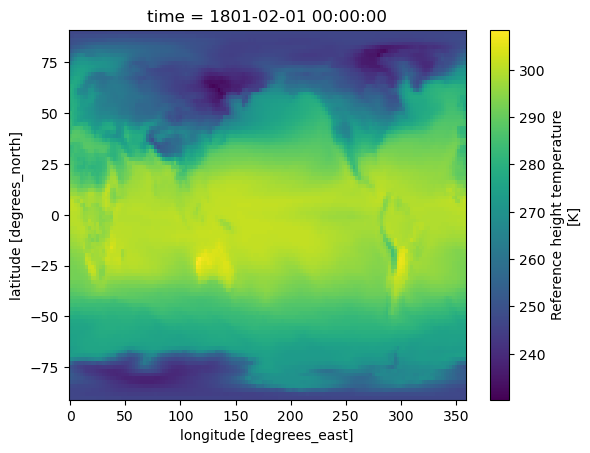
Customize plot#
set the figure size
set the projection
fig = plt.figure(1, figsize=[30,13])

# Set the projection to use for plotting
ax = plt.subplot(1, 1, 1, projection=ccrs.PlateCarree())
ax.coastlines()

# Pass ax as an argument when plotting. Here we assume data is in the same coordinate reference system than the projection chosen for plotting
# isel allows to select by indices instead of the time values
ds['TREFHT'].isel(time=0).squeeze().plot.pcolormesh(ax=ax, cmap='coolwarm')
<cartopy.mpl.geocollection.GeoQuadMesh at 0x6ffc30aa38c0>
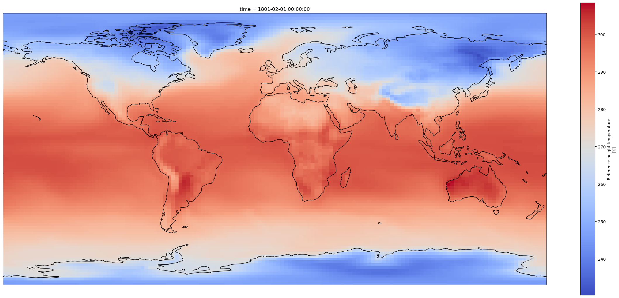
Change plotting projection#
fig = plt.figure(1, figsize=[8, 8])

# We're using cartopy and are plotting in Orthographic projection
# (see documentation on cartopy)
ax = plt.subplot(1, 1, 1, projection=ccrs.Orthographic(0, 90))
ax.coastlines()

# We need to project our data to the new Orthographic projection and for this we use `transform`.
# we set the original data projection in transform (here PlateCarree)
ds['TREFHT'].isel(time=0).squeeze().plot(ax=ax, transform=ccrs.PlateCarree(), cmap='coolwarm')

# One way to customize your title
plt.title(ds.time.values[0].strftime("%B %Y"), fontsize=18)
Text(0.5, 1.0, 'February 1801')